Ssa (singular spectrum analisys)

We have some data. Our goal for today would be to find the cyclical pattern that the data presents.

Problem description

To give one use case for this, let’s say we work for an online store company. We’re planning to increase our sales by promoting (through advertising) some products, discounts or special offers. The end goal would be to have people that see ads, buy these stuff. Someone seeing an ad, then making a purchase is called a conversion.

Unfortunately, the number of conversions happen irregularly (we’re not seeing each hour roughly the same amount of conversions). At the same time though, the conversions we’re seeing have a clear pattern, one of which we’ve identified by looking at the charts is the day/night pattern. This makes sense: people usually buy during the day and not that often at night.

Obiously day / night is not the only pattern, there are potentially more, which look when summed up like complex looking shapes.

Our problem is identifying all these patterns, for:

• tailoring our marketing campaing by spending more on the intervals with high conversion rate, and stop the campaing on the slughish intervals.
• understand the main conversion driving factors for our clients (holidays, vacation periods, etc..?)
• understand our clients. We’ve assumed day / night is a pattern but the cycles for days don’t line up with our local time. This may be because:
  • our customers come from a different part of the world
  • it’s not a day / night but a after-hours / morning-hours one
  • others..

I hope I’ve convinced you that exactly knowing the caracteristics of the patterns in our data is of great help.

Generate data

Normally, any data that we work with has 3 main components:

• Trend (generically going up, or generically going down). The trend is an overall shape that the data seems to follow. It may be a straight line, or a parabola, or some other shape, whose domain spans all the data we have.
• Seasonality (the actual pattern we are looking for). This is a periodical function, that spans multiple cycles in our dataset (like the day / night cycle, winter / summer, full moon / no moon, fiscal Q1 / Q2 / Q3 / Q4, etc..)
• Noise - Some random stuff that we want to ignore, but which is already contained in the data.

So we assume, of the bat, that most data has the following structure:

\[f(t) = trend(t) + seasonality(t) + noise(t)\]

We’re initerested in seasonality but finding that implies actually finding the other two components (because the trend is usually a low polinomyal regression over $trend(t) + noise(t)$). So we will be exploring (one way) of decomposing our data into the three parts above.

Definining the main components of the data

In our case, we will be generating our toy data using the following definitions:

\[trend(t) = .001 * t ^ 2\] \[seasonality(t) = sin(\frac{\pi}{4}) + 5 * cos(\frac{\pi}{2})\] \[noise(t) = Random(0, 5)\] \[f(t) = 0.001*t^2 + sing(\frac{\pi}{4}) + 5 * cos(\frac{\pi}{2}) + Random(0, 5)\]

The trend is the overall pattern of the data. The trend is not about repeating patterns but about the generic direction.

import numpy as np
import pandas as pd
from matplotlib import pyplot as plt
import math

Code

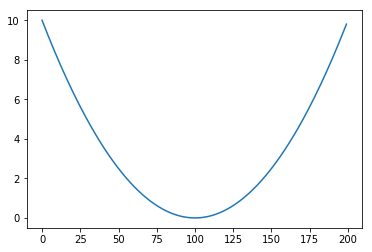
def trend(t):
    """
    Function that for a certain t returns a quadratic function applied on that point. 
    """
    return 0.001 * t ** 2

T = list(range(-100, 100))
Trend = [trend(t) for t in T]
plt.plot(Trend)

Then we add two periodical function to the mix (essentialy these are what we’re after)

Code

def apply(func, T):
    """
    Mapping function. Applies to all the values in T the function func and returns a list with the results.
    """
    return [func(t) for t in T]

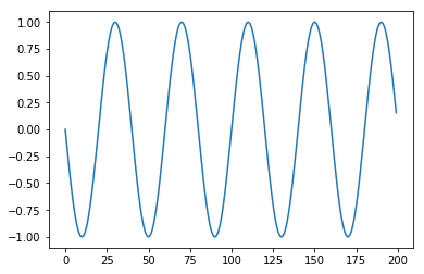
def period_1(t, period = 20):
    return math.sin(math.pi * t / period)

plt.plot(apply(period_1, T))

Code

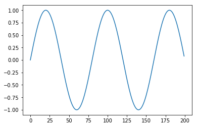
def period_2(t, period = 40):
    return math.cos(math.pi * t / period)

plt.plot(apply(period_2, T))

And add in some noise to make the problem hard.

Code

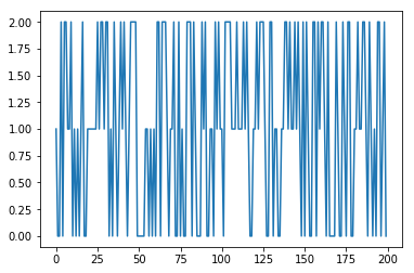
def noise(t):
    return np.random.randint(0, 3)

plt.plot(apply(noise, T))

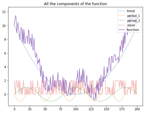
Our final function is then:

\[f(t) = trend(t) + period_1(t) + period_2(t) + noise(t) = 0.001*t^2 + sing(\frac{\pi}{4}) + 5 * cos(\frac{\pi}{2}) + Random(0, 5)\]

def f(t):
    return trend(t) + period_1(t) + period_2(t) + noise(t)

f(10)

1.8071067811865476

Code

plt.figure(figsize=(8, 6))
plt.plot(apply(trend, T), alpha=0.4)
plt.plot(apply(period_1, T), alpha=0.4)
plt.plot(apply(period_2, T), alpha=0.4)
plt.plot(apply(noise, T), alpha=0.4)
plt.plot(apply(f, T))
plt.legend(["trend", "period_1", "period_2", "noise", "function"], loc='upper right')
plt.title("All the components of the function")

F = np.array(apply(f, T))
F.shape

(200,)

Decompose that!!

Idea of the approach

We’ve said that we assume, most data to have the following structure:

\[f(t) = trend(t) + seasonality(t) + noise(t)\]

Some notes:

• Even thought trend is seen in this formulation as something different from seasionality, it can be (and usually is, given data that spans enough time), the trend ca also be a seasionality component, althoug one with a very long periodicity.
• Even though seasonality is seen as a single factor, it can actually be a composition of multiple periodic functions, with different frequency and amplitudes. For example in case of some spending data, we can have day/night patterns, Q1 / Q4 patterns, holiday and year-on-year patterns at the same time. Some of these components will have a longer cycle, some smaller. They all constitute seasonality factors because we should have (by definition) multiple cycles (they manifest repeatably) in our data.
• Even though noise(t) is seen in this formulation as something different from seasionality, like a random process, is can also be some seasionality component, although a very short one (with minute / second long frequency). Or even in the case where noise is trully random, we can simulate it using some really short frequency seasionality components added togheter.

Having said that, we will try to do the following:

• model $f(t)$ as a sum of periodic functions (components)
• find (heuristical) ways to group these components into the 3 categories (trend, seasonality, noise)
  • low periodicity means trend, medium periodicity means seasionality, others are noise
  • for example, one heuristic would be to group as trend all the components that have a period greather than the timespan of the data we have.

So \(f(t) = \sum_{period=long}{component_i(t)} + \sum_{period=medium}{component_j(t)} + \sum_{period=short}{component_k(t)}\)

Choosing an approach

We will be using here the Singular Spectrum Analisys (SSA) which is based on Singular Value Decomposition (SVD).

• the shape above is really similar to a Fourier Transform decomposition into basic trigonometric functions. Although we won’t be using it, a Fourier decomposition can be used to replicate this. It’s called Fourier Analisys (FA).

The reason to use SSA over FA is

due to the fact that a single pair of data-adaptive SSA eigenmodes often will capture better the basic periodicity of an oscillatory mode than methods with fixed basis functions, such as the sines and cosines used in the Fourier transform.
(quote)

This roughly sais that often SSA works better because it has a more complex modeling technique (based on eigenvalues) compared to Fourier Analisys (which is trignometrical functions based).

It’s possible that the practical reason is that FA will yield to multiple basic components compared to SSA and thus:

• grouping them into trend, seasionality and noise will be harder
• interpreting the FA may be more difficult

SSA (Singular Spectrum analisys) EDA

Main algorithm description of SSA

You will find bellow a lot of math notation but we’ll going to do this step by step in code after the next section. I’m including this here just to have an outline of what we’re going to do next. It’s ok if you only get 30-40% of what this means.

Hopefully, after we go through the actual implementation, comming back to this will gruadually start to make more sense.

Step 1: Embedding

Form the trajectory matrix of the series $\mathbf X$ , which is the $L * K$

\[\displaystyle \mathbf {X} =[X_{1}:\ldots :X_{K}]=(x_{ij})_{i,j=1}^{L,K}={\begin{bmatrix}x_{1}&x_{2}&x_{3}&\ldots &x_{K}\\x_{2}&x_{3}&x_{4}&\ldots &x_{K+1}\\x_{3}&x_{4}&x_{5}&\ldots &x_{K+2}\\\vdots &\vdots &\vdots &\ddots &\vdots \\x_{L}&x_{L+1}&x_{L+2}&\ldots &x_{N}\\\end{bmatrix}}\]

where \(X_{i}=(x_{i},\ldots ,x_{i+L-1})^{\mathrm {T}}\;\quad (1\leq i\leq K)\) are lagged vectors of size $L$.

The matrix $\mathbf {X}$ is a Hankel matrix which means that $\mathbf {X}$ has equal elements $x_{ij}$ on the anti-diagonals $i+j=\,{\rm {const}}$.

Step 2: Singular Value Decomposition (SVD)

Perform the singular value decomposition (SVD) of the trajectory matrix $\mathbf {X}$. Set ${\mathbf {S}}={\mathbf {X}}{\mathbf {X}}^{\mathrm {T}}$ and denote by:

• $\lambda _{1},\ldots ,\lambda _{L}$ the eigenvalues of $\mathbf {S}$ taken in the decreasing order of magnitude ($\lambda _{1}\geq \ldots \geq \lambda _{L}\geq 0$)
• $U_{1},\ldots ,U_{L}$ the orthonormal system of the eigenvectors of the matrix $\mathbf {S}$ corresponding to these eigenvalues.
• $V_{i}={\mathbf {X}}^{\mathrm {T}}U_{i}/{\sqrt {\lambda _{i}}} (i=1,\ldots ,d)$, where $d={\mathop {\mathrm {rank}}}({\mathbf {X}})=\max{i,\ {\mbox{such that}}\ \lambda _{i}>0}$ (note that $d=L$ for a typical real-life series)

In this notation, the SVD of the trajectory matrix $\mathbf {X}$ can be written as

\({\mathbf {X}}={\mathbf {X}}_{1}+\ldots +{\mathbf {X}}_{d}\), where

\({\mathbf {X}}_{i}={\sqrt {\lambda _{i}}}U_{i}V_{i}^{\mathrm {T}}\) are matrices having rank 1; these are called elementary matrices.

The collection ($\sqrt {\lambda_{i}},U_{i},V_{i}$) will be called the $i$th eigentriple (abbreviated as ET) of the SVD. Vectors $U_{i}$ are the left singular vectors of the matrix $\mathbf {X}$ , numbers ${\sqrt {\lambda_{i}}}$ are the singular values and provide the singular spectrum of $\mathbf {X}$ ; this gives the name to SSA. Vectors ${\sqrt {\lambda_{i}}}V_{i}={\mathbf {X}}^{\mathrm {T}}U_{i}$ are called vectors of principal components (PCs).

Step 3: Eigentriple grouping

Partition the set of indices ${1,\ldots ,d}$ into $m$ disjoint subsets $I_{1},\ldots ,I_{m}$.

Let $I={i_{1},\ldots ,i_{p}}$. Then the resultant matrix \({\mathbf {X}}_{I}\) corresponding to the group $I$ is defined as \({\mathbf {X}}_{I}={\mathbf {X}}_{i_{1}}+\ldots +{\mathbf {X}}_{i_{p}}\). The resultant matrices are computed for the groups $I=I_{1},\ldots ,I_{m}$ and the grouped SVD expansion of $\mathbf {X}$ can now be written as

\[{\mathbf {X}}={\mathbf {X}}_{I_{1}}+\ldots +{\mathbf {X}}_{I_{m}}\]

Step 4: Diagonal averaging

Each matrix \({\mathbf {X}}_{I_{j}}\) of the grouped decomposition is hankelized and then the obtained Hankel matrix is transformed into a new series of length $N$ using the one-to-one correspondence between Hankel matrices and time series. Diagonal averaging applied to a resultant matrix \({\mathbf {X}}_{I_{k}}\) produces a reconstructed series

\[\widetilde {\mathbb {X}}^{(k)}=(\widetilde {x}_{1}^{(k)},\ldots ,\widetilde {x}_{N}^{(k)})\]

In this way, the initial series $x_1,\ldots,x_N$ is decomposed into a sum of \({\displaystyle m}m\) reconstructed subseries:

\(x_{n}=\sum \limits _{k=1}^{m}\widetilde {x}_{n}^{(k)}\ \ (n=1,2,\ldots ,N)\) This decomposition is the main result of the SSA algorithm. The decomposition is meaningful if each reconstructed subseries could be classified as a part of either trend or some periodic component or noise.

Actual implementation

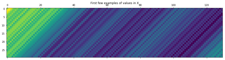
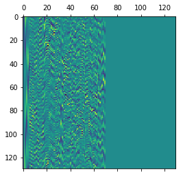
Step 1: Embedding

• compute the trajectory matrix (autocorrelation matrix). The matrix is column wise a stack of windows of size L over all the data. So:
  • column 1 is $f_0 .. f_{L-1}$
  • column 2 is $f_1 .. f_L$
  • column 3 is $f_2 .. f_{L+1}$
  • ..

\[\mathbf{X} = \begin{bmatrix} f_0 & f_1 & f_2 & f_3 &\ldots & f_{N-L} \\ f_1 & f_2 & f_3 & f_4 &\ldots & f_{N-L+1} \\ f_2 & f_3 & f_4 & f_5 &\ldots & f_{N-L+2} \\ \vdots & \vdots & \vdots & \vdots & \ddots & \vdots \\ f_{L-1} & f_{L} & f_{L+1} & f_{L+2} & \ldots & f_{N-1} \\ \end{bmatrix}\]

• this is also called a Hankel matrix

L = 70 # window size
N = len(T) # number of observations
X = np.array([F[offset:(offset+L)] for offset in range(0, N - L)]).T

Code

plt.matshow(X[:30])
plt.title("First few examples of values in X");

An alternative way of composing the above is as follows (using np.column_stack)

X_ = np.column_stack([F[offset:(offset+L)] for offset in range(0, N - L)])
np.allclose(X, X_)

True

Step 2: Applying SVD

The main idea of this step is to have find $i$ elementarry matrices that exhibit the following property:

\({\mathbf {X}}={\mathbf {X}}_{1}+\ldots +{\mathbf {X}}_{d}\),

The wikipedia way

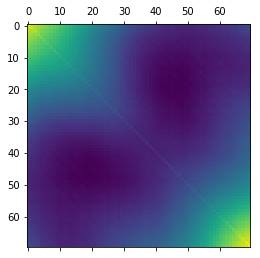
On the Step 2 we are required to compute the $X*X^T$.

Note: On Python 3 we can use the @ operator for doing a matrix multiplication. This should be equivalent to doing np.matmul

np.allclose(X @ X.T, np.matmul(X, X.T))

True

We’re going to print the $X*X^T$ matrix to have a visual idea of what that looks like.

Code

plt.matshow(X @ X.T)

U, S, _V_t = np.linalg.svd(X @ X.T)
_V = _V_t.T

U.shape, S.shape, _V.shape

((70, 70), (70,), (70, 70))

Now S consists of L eigenvalues $\lambda _{1},\ldots ,\lambda _{L}$ of $\mathbf {S}$ taken in the decreasing order of magnitude ($\lambda _{1}\geq \ldots \geq \lambda _{L}\geq 0$)

Code

plt.plot(S[:10])

If we follow the algorithm, we should be constructing $V$ as follows:

• \(V_{i}={\mathbf {X}}^{\mathrm {T}}U_{i}/{\sqrt {\lambda_{i}}} (i=1,\ldots ,d)\), where \(d={\mathop {\mathrm {rank}}}({\mathbf {X}})=\max\{i,\ {\mbox{such that}}\ \lambda_{i}>0\}\) (note that $d=L$ for a typical real-life series)

The $rank$ of the matrix is the cardinal of the last index $i$, where number $S_i > 0$. If the rank is lower than the dimentions of $U$ this means that the matrix can be decomposed without loss into fewer dimensions. In most real world examples we’re not that lucky, and $rank == U.shape[0]$

rank = np.where(S > 0)[0][-1] + 1
rank

70

Now let’s reconstruct the V matrix as in the wiki algorithm.

V = np.zeros(shape=(130, 130))
for column in range(rank):
    V[:, column] = (X.T@U[:, column]) / np.sqrt(S[column])
plt.matshow(V)

Numpy decomposes our $\Sigma$ value into a 1D array of singular values, but mathematically, $\Sigma$ should have the shape (U.shape[-1], V.shape[0]) for the computation to be well defined.

As such we will recompose the propper matrix $\Sigma$ using the function bellow.

def inflate_s(U, S, V):
    """
    Function that takes in the S value returned by 
    np.linalg.svd decomposition and reconstructs the mathematical
    diagonal matrix that it represents. 
    """
    _S = np.zeros(shape=(U.shape[-1], V.T.shape[0]))
    _S[:U.shape[1],:U.shape[1]] = np.diag(S)
    return _S

_S = inflate_s(U, S, V)
plt.matshow(_S)

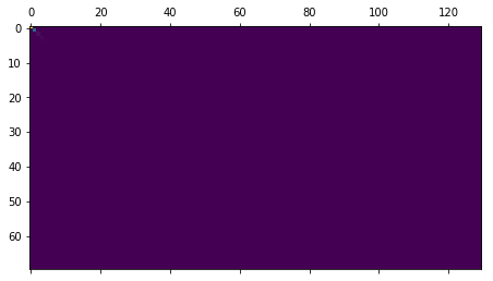
While $\Sigma$ looks empty, if you look closely you can barely see on the (0, 0), (1, 1) and (2, 2) - the first diagonal- some non zero values. So it’s working properly.

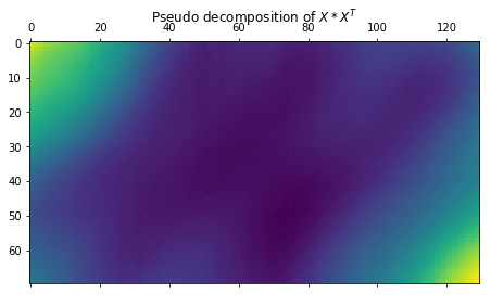
Now let’s see what the actual $U * \Sigma * V^T$ looks like. It will obviously not be the same matrix reconstruction as $X$ since we’r using $U$ and $\Sigma$ from the decomposition of the matrix $X * X_T$, and V is a derivative of these two ($U$ and $\Sigma$)

Code

plt.matshow(U @ _S @ V.T)
plt.title(r"Pseudo decomposition of $X * X^T$")
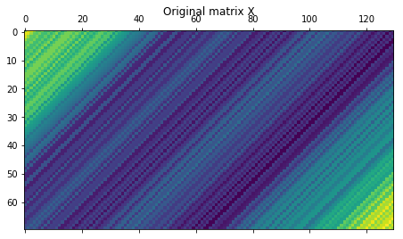
plt.matshow(X)
plt.title(r"Original matrix X")

Now let’s compute the elementary matrices \({\mathbf {X}}_{i}={\sqrt {\lambda_{i}}}U_{i}V_{i}^{\mathrm {T}}\)

_X = np.zeros((rank, X.shape[0], X.shape[1]))
for i in range(rank):
    _X[i] = (np.sqrt(S[i])*U[:, [i]])@V[:, [i]].T

Notice that in this formulation, we are doing a regular matrix multiplication between U[:, i] and V[:, i].T but this is equivalent on doing an outer product between U[:, i] and V[:, i].

In the check bellow we are using [i] indexing on columns so we end up with matrices rather than vectors that we can then transpose via .T otherwise transposing a vector in numpy doesn’t have any effect (so not our intended 1 column and many rows shape for V). This is rather an API quirk.

np.allclose(
    np.outer(U[:, i], V[:, i]),
    U[:, [i]] @ V[:, [i]].T
)

True

Code

def is_square(integer):
    """
    This function is harder to write (correctly) than I have previously imagined.
    
    # https://stackoverflow.com/questions/2489435/check-if-a-number-is-a-perfect-square
    """
    root = math.sqrt(integer)
    return integer == int(root + 0.5) ** 2

def prepare_axis(ax, i):
    ax.get_xaxis().set_visible(False)
    ax.set_ylabel(f"{i}")
    ax.set_yticks([])
    ax.set_yticklabels([])
    return ax

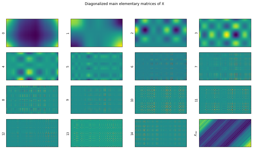
def show_elementary_matrices(X_elem, rank, max_matices_to_show = 9):
    figure_max = 15
    dims_to_show = min((figure_max, max_matices_to_show, rank))

    axes_needed = dims_to_show + 1
    n_rows = int(np.sqrt(axes_needed)) if is_square(axes_needed) else int(np.ceil(np.sqrt(axes_needed)))
    n_cols = int(np.ceil(np.sqrt(axes_needed)))

    fig, axs = plt.subplots(n_rows, n_cols, figsize=(15, 8))
    axs = [prepare_axis(ax, i) for i, ax in enumerate(axs.flatten())];

    for i, s_i in enumerate(S[:dims_to_show]):
        axs[i].matshow(X_elem[i])
        axs[i].get_xaxis().set_visible(False)
        axs[i].set_ylabel(f"{i}")
        axs[i].set_yticks([])
        axs[i].set_yticklabels([])

    X_rec = np.sum(X_elem, axis=0)
    axs[-1].matshow(X_rec)
    axs[-1].get_xaxis().set_visible(False)
    axs[-1].set_ylabel("$X_{rec}$")
    axs[-1].set_yticks([])
    axs[-1].set_yticklabels([''])
    fig.suptitle("Diagonalized main elementary matrices of X")

show_elementary_matrices(X_elem=_X, rank=rank, max_matices_to_show=15)

We’re expecting that the elementarry matrices in _X will all sum up to X.

np.allclose(np.sum(_X, axis=0), X, atol=1e-10)

True

So the difference between them is not significant! We’re all set.

Code

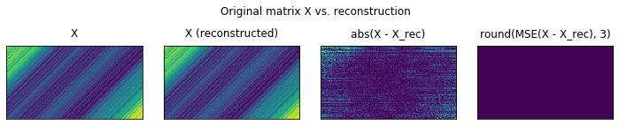
def plot_original_vs_rec(X, X_elem):
    fig, (ax1, ax2, ax3, ax4) = plt.subplots(1, 4, figsize=(10, 2.5))
    ax1.matshow(X)
    ax1.set_title("X")
    ax1.get_xaxis().set_visible(False)
    ax1.get_yaxis().set_visible(False)

    X_rec = np.sum(X_elem, axis=0)
    ax2.matshow(X_rec)
    ax2.set_title("X (reconstructed)")
    ax2.get_xaxis().set_visible(False)
    ax2.get_yaxis().set_visible(False)


    ax3.matshow(np.abs(X - X_rec))
    ax3.set_title("abs(X - X_rec)")
    ax3.get_xaxis().set_visible(False)
    ax3.get_yaxis().set_visible(False)


    ax4.matshow(np.round(np.sqrt(np.power(X - X_rec, 2)), 3))
    ax4.set_title("round(MSE(X - X_rec), 3)")
    ax4.get_xaxis().set_visible(False)
    ax4.get_yaxis().set_visible(False)

    fig.suptitle("Original matrix X vs. reconstruction")
    fig.tight_layout()

plot_original_vs_rec(X, _X)

The kaggle way

There is also another way of decomposing $X$ into i elementarry matrices $X_i$ that can be summed up to $X$, presented on this kaggle kernel.

This basically avoids doing the $X * X^T$ decomposition through SVD in order to get to a series of elementary matrices $X_i$ and in turn opt for directly decomposing $X$ into $U$, $\Sigma$ and $V$ which will be used to construct the $X_i$ elementarry matrices.

This has one big advantage in that the result $X$ is closer to the actual values of $X_i$ (fewer steps) and on the whole:

• reduce the number of mistakes that can be done
• reduce the possiblity of floating point operations underflows
• is more explicit and easyer to understand
• eliminates a lot of mathemathical machinery that is not really obvoius as to why they are needed (remember the convoluted way in which we’ve build $V$ using the wikipedia way).

Remember that this step is only about finding suitable $X_i$ such as:

\[{\mathbf {X}}={\mathbf {X}}_{1}+\ldots +{\mathbf {X}}_{d}\]

We first deconstruct X in $U * \Sigma * V.T$ through SVD.

U, S, V_T = np.linalg.svd(X)
V = V_T.T
U.shape, S.shape, V.shape

((70, 70), (70,), (130, 130))

Now our elementary matrices are, \(X_i = \sigma_i U_i V_i^{\text{T}}\)

and,

\[X = \sum_{i=0}^{d-1}X_i\]

• $\sigma_i$ is the i-th singular value of $\Sigma$. This means S[i] in numpy notation (because numpy’s SVD returns a vector for S, with the non zero values of the diagonal - remember that S is a diagnoal matrix).
• $U_i$ is the column i of U
• $V^T_i$ is the column i of $V^T$
• the product between $U_i$ and $V^T_i$ is an outer product
• d is the rank of the matrix $\mathbf{X}$, and is the maximum value of $i$ such that $\sigma_i > 0$.

(Note: for noisy real-world time series data, the S matrix is likely to have rank=𝐿 dimensions.)

In order to replicate the formula, we will have to construct multiple separable matices $X_i$ that we will then need to sum up. We will have as many such separable matrices as we have singular non-zero values in $S$ (aka rank d).

You can compute the rank using np.linalg.matrix_rank(X) but that internally computes the SVD decomposition all over again and as we’ve seen above we can compute the rank using plain Python with the same result.

d = np.where(S > 0)[0][-1] + 1
assert d == np.linalg.matrix_rank(X)

X_ = np.array([S[i] * np.outer(U[:, i], V[:, i]) for i in range(d)])
X_.shape

(70, 70, 130)

Code

show_elementary_matrices(X_elem=X_, rank=d, max_matices_to_show=15)

Let’s show in more detail the result of the reconstructions.

Code

plot_original_vs_rec(X, X_)

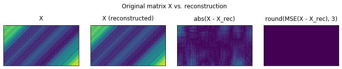
We observe that in actual fact, there are some errors in the reconstruction, but the total MSE over all pixels is null. This is given by the fact, that the errors are subunitary, on the order of 1e-10. Raising by the power 2 makes these number even furter small.

We could have illustrated this by rounding as well (like we did bellow). Notice that we now have only 0s.

np.round((X - X_rec)[:10, :], 2)

array([[0., 0., 0., ..., 0., 0., 0.],
       [0., 0., 0., ..., 0., 0., 0.],
       [0., 0., 0., ..., 0., 0., 0.],
       ...,
       [0., 0., 0., ..., 0., 0., 0.],
       [0., 0., 0., ..., 0., 0., 0.],
       [0., 0., 0., ..., 0., 0., 0.]])

Comparing the two elementary matrices sets

So by now we have to ways of decomposing X into a sum of elemenatary matrices and I’m wondering weather they result in the same values.

np.allclose(_X, X_)

True

It seems so! To be honest, it’s not obvious to me why the two are equivalent, but I’ll just take this conclusion based on this experimental evidence.

So whichever route you choose (wikipedia or kaggle) both will yield the same decomposition of X.

Understanting each elementary matrices contribution

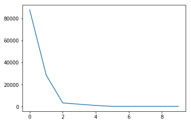
We expect that the values in S be sorted descending (the first component being the dominant one)

Code

plt.bar(np.arange(d),S[:d])

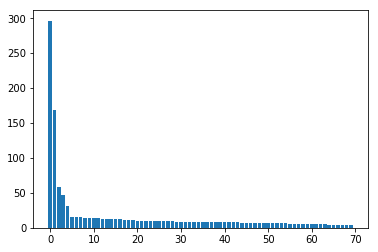
S[:d]

array([296.38093887, 169.08832106,  57.86482217,  46.40141   ,
        31.90894601,  15.34198554,  14.86843714,  14.78694165,
        14.5247375 ,  14.37088651,  13.58001463,  13.43212073,
        12.48453521,  12.38210474,  12.23913403,  12.19359197,
        12.06379809,  11.84667796,  10.87244838,  10.54201025,
        10.4285727 ,  10.25184033,  10.1185066 ,   9.87839322,
         9.66298264,   9.62024667,   9.52666637,   9.34031991,
         9.08076815,   8.98204041,   8.88240115,   8.79184386,
         8.69677049,   8.6275053 ,   8.57455309,   8.32935018,
         8.3016696 ,   8.19605236,   8.16795458,   8.0082251 ,
         7.87639454,   7.84820178,   7.78861214,   7.76982839,
         7.52879927,   7.29338437,   7.21568859,   7.10035755,
         6.96965055,   6.87384928,   6.65348868,   6.59733372,
         6.47399648,   6.32487688,   6.20118721,   5.96992107,
         5.836588  ,   5.73879453,   5.71891451,   5.63213598,
         5.4930785 ,   5.3414355 ,   5.30227011,   4.99551775,
         4.58242342,   4.4556975 ,   3.91478919,   3.90050813,
         3.44812975,   3.36613955])

Math shows that \(\lvert\lvert \mathbf{X} \rvert\rvert_{\text{F}}^2 = \sum_{i=0}^{d-1} \sigma_i^2\) i.e. the squared Frobenius norm of the trajectory matrix is equal to the sum of the squared singular values.

np.allclose(np.linalg.norm(X) ** 2, np.sum(S[:d] ** 2))

True

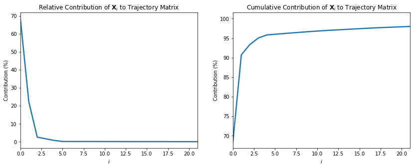
This suggests that we can take the ratio $\sigma_i^2 / \lvert\lvert \mathbf{X} \rvert\rvert_{\text{F}}^2$ as a measure of the contribution that the elementary matrix $\mathbf{X}_i$ makes in the expansion of the trajectory matrix $X$.

If we’re only insterested on the order of the components and their magnitude we could get away without dividing on the norm, as it is the same computation on all the sigular values.

Code

s_sumsq = (S**2).sum()
fig, ax = plt.subplots(1, 2, figsize=(14,5))
number_of_components_to_show = 20

ax[0].plot(S**2 / s_sumsq * 100, lw=2.5)
ax[0].set_xlim(0,number_of_components_to_show + 1)
ax[0].set_title("Relative Contribution of $\mathbf{X}_i$ to Trajectory Matrix")
ax[0].set_xlabel("$i$")
ax[0].set_ylabel("Contribution (%)")
ax[1].plot((S**2).cumsum() / s_sumsq * 100, lw=2.5)
ax[1].set_xlim(0,number_of_components_to_show + 1)
ax[1].set_title("Cumulative Contribution of $\mathbf{X}_i$ to Trajectory Matrix")
ax[1].set_xlabel("$i$")
ax[1].set_ylabel("Contribution (%)");

def cummulative_contributions(S):
    return (S**2).cumsum() / (S**2).sum()

def relevant_elements(S, variance = 0.99):
    """
    Returns the elementary elements X_i needed to ensure that we retain the given degree of variance.
    S is the singular value matrix returned by the svd procedure while decomposing X.
    """
    cumm_contributions = cummulative_contributions(S)
    last_contributing_element = np.where(cumm_contributions > variance)[0][0] + 1
    return np.arange(last_contributing_element)

relevants = relevant_elements(S, variance=0.99)
cummulative_contributions(S)[relevants]

array([0.68453083, 0.90733315, 0.93342601, 0.95020458, 0.95813904,
       0.95997327, 0.96169603, 0.96339995, 0.96504398, 0.96665336,
       0.96809048, 0.96949647, 0.97071108, 0.97190584, 0.97307317,
       0.97423183, 0.97536595, 0.97645962, 0.97738081, 0.97824685,
       0.97909436, 0.97991338, 0.98071124, 0.98147168, 0.98219931,
       0.98292053, 0.98362778, 0.98430764, 0.98495023, 0.98557893,
       0.98619376, 0.98679611, 0.98738551, 0.98796556, 0.9885385 ,
       0.98907915, 0.98961621, 0.9901397 ])

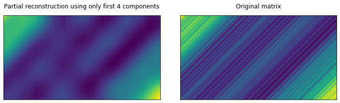
Partially reconstructing X, by only using the top 4 components

We see that only the first 4 components (maybe even 3) contribute some meaningfull values to the reconstruction of $X$. The other singular values in S (and thus respective elementary matrices $X_i$ could be ignored).

Let’s see what happens if we remove them and only reconstruct X from the first few elementary matrices.

Code

fig, (ax1, ax3) = plt.subplots(1, 2, figsize=(10, 6))

def no_axis(ax):
    ax.get_xaxis().set_visible(False)
    ax.get_yaxis().set_visible(False)
    return ax

ax1, ax3 = no_axis(ax1), no_axis(ax3)

compomnents_to_use = 4
ax1.matshow(np.sum(X_[:compomnents_to_use], axis=0))
ax1.set_title(f"Partial reconstruction using only first {compomnents_to_use} components")

ax3.matshow(X)
ax3.set_title("Original matrix")

fig.tight_layout();

Let’s also show an animation of that looks like for more components.

Code

from matplotlib import animation, rc
from IPython.display import HTML

fig, (ax1, ax3) = plt.subplots(1, 2, figsize=(10, 5))
ax1, ax3 = no_axis(ax1), no_axis(ax3)


plot = ax1.matshow(np.sum(X_[:d], axis=0))
ax1.set_title(f"Partial reconstruction using only first {1} components")

ax3.matshow(X)
ax3.set_title("Original matrix")

fig.tight_layout()

def animate(i, plot):
    ax1.set_title(f"Recon. with {i} comp.")
    plot.set_data(np.sum(X_[:i], axis=0))
    return [plot]

anim = animation.FuncAnimation(fig, animate, fargs=(plot,), frames=min(100, d), interval=200, blit=False)
display(HTML(anim.to_html5_video()))
plt.close()

Step4: Diagonal averaging

The wikipedia article and the kaggle kernel diverge somewhat at this point. There are 3 steps that still need to be done:

1. Group the elementary matrices into disjoint groups, summing the groups into a new set of (still) elementary matrices

\[\begin{align*} \mathbf{X} & = \sum_{k \in \mathcal{S}}\mathbf{X}_k + \sum_{l \in \mathcal{T}}\mathbf{X}_l + \ldots \\ & = \sum_j \mathbf{X}^{(j)} \end{align*}\]

1. Hankelise the elementary matrices by diagonal averaging.
2. Derive the timeseries components from the Henkel matrices.

While wikipedia suggest doing 1., 2., 3. the kaggle kernel actually does 2., 3., 1. (so it henkelises first, then extracts the timeseries and then it groups).

It’s unclear what the grouping strategy is for the wikipedia article, so we’ll stick to 2., 3., 1.

Henkelisation of the elementary matrices

We need to reconstruct a Henkel matrix (the matrix with diagonal lines) as this is the thing we’ve started the deconstruction from, and as we’ve seen in the animation above adding the elementary matrices leads progressively to a henkel matrix.

The problem is that we’d like to understand what these elementary matrices represent as a timeseries component.

From a hankel matrix, you can extract the timeseries (row[0] concat. column[-1]). To see why this works, remember the shape we gave to X:

\[\displaystyle \mathbf {X} =[X_{1}:\ldots :X_{K}]=(x_{ij})_{i,j=1}^{L,K}={\begin{bmatrix}x_{1}&x_{2}&x_{3}&\ldots &x_{K}\\x_{2}&x_{3}&x_{4}&\ldots &x_{K+1}\\x_{3}&x_{4}&x_{5}&\ldots &x_{K+2}\\\vdots &\vdots &\vdots &\ddots &\vdots \\x_{L}&x_{L+1}&x_{L+2}&\ldots &x_{N}\\\end{bmatrix}}\]

To extract $[x_{1}:\ldots :x_{N}]$ from the henkel matrix $X$ you just take X[0, :] and concat that with X[1:, -1].

It’s because of this that we actually seek to force the elementary matrices to be henkel matrices. This can be done using a process called diagonal averaging where each values represents the mean of all the elements of its corresponding diagonal.

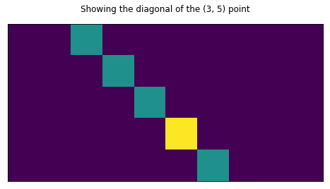
A simple and not so efficient way of computing the indices of the elements that compose the diagonal of a certain point is shown bellow

Code

elem, shape = (3, 5), (5, 10)

def diagonal(elem, shape):
    """
    Computes all the elements that compose the diagonal in which 
    the given point (x, y) is a member of.
    """
    def _is_valid(i, j):
        return (0<=i<n) and (0<=j<m)
    
    n, m = shape
    x, y = elem
     
    j_offset = abs(x - y)
    for i in range(max(n, m)):
        j = i + j_offset
        if _is_valid(i, j):
            yield i, j

def numpy_indices(diagonal_gen):
    """
    Just takes the [(x1,y1), ..] generator and reshapes it into [[x1, ...], [y1, ...]] 
    so these can be plugged into a numpy array index
    """
    return tuple(zip(*diagonal_gen))

a = np.zeros(shape)
a[numpy_indices(diagonal(elem, shape))] = 1
a[elem] = 2

plt.matshow(a)
plt.title(f"Showing the diagonal of the {elem} point")
plt.xticks([]), plt.yticks([]);

It’s maybe easyer to show these in a short animation

Code

elem, shape = (2, 2), (5, 10)

def init():
    a = np.zeros(shape)
    a[numpy_indices(diagonal(elem, shape))] = 1
    a[elem] = 2

    fig, ax = plt.subplots(figsize=(8, 5))
    plot = ax.matshow(a)
    plt.title(f"Showing the diagonal of the {elem} point")
    plt.xticks([]), plt.yticks([]);
    return fig, ax, plot
    
def animate(i, plot):
    _elem = (elem[0], elem[1] + i)
    
    a = np.zeros(shape)
    a[numpy_indices(diagonal(_elem, shape))] = 1
    a[_elem] = 2
    
    ax.set_title(f"Diagonal of element {_elem}")
    plot.set_data(a)
    return [plot]

fig, ax, plot = init()
anim = animation.FuncAnimation(fig, animate, fargs=(plot,), frames=8, interval=500, blit=False)
display(HTML(anim.to_html5_video()))
plt.close()

What we actually want is to compute the antidiagonal. Which is…

Code

elem, shape = (2, 0), (5, 10)

def antidiagonal(elem, shape):
    """
    Computes the elements of the antidiagonal
    """
    def _is_valid(i, j):
        return (0<=i<n) and (0<=j<m)
    
    (x, y), (n, m) = elem, shape
    tot = x + y
    for i in range(tot + 1):
        j = tot - i
        if _is_valid(i, j):
            yield i, j

def init():
    a = np.zeros(shape)
    a[numpy_indices(diagonal(elem, shape))] = 1
    a[elem] = 2

    fig, ax = plt.subplots(figsize=(8, 5))
    plot = ax.matshow(a)
    plt.title(f"Showing the diagonal of the {elem} point")
    plt.xticks([]), plt.yticks([]);
    return fig, ax, plot

def animate(i, plot):
    _elem = (elem[0], elem[1] + i)
    
    a = np.zeros(shape)
    a[numpy_indices(antidiagonal(_elem, shape))] = 1
    a[_elem] = 2
    
    ax.set_title(f"Antidiagonal of element {_elem}")
    plot.set_data(a)
    return [plot]

fig, ax, plot = init()
anim = animation.FuncAnimation(fig, animate, fargs=(plot,), frames=10, interval=500, blit=False)
display(HTML(anim.to_html5_video()))
plt.close()

The henkelisation procedure is the following:

• we will scan all the (i,j) elements of the matrix $X_i$
• we will compute the indices D of the antidiagonal of which (i,j) is an element of
• we will compute the mean of the values of the elements found on D
• set the mean above as the (i,j) values in the henkelized $X_{hat}$ matrix.

def henkelize(X):
    """
    Henkelisation procedure for the given matrix X.
    Returns a matrix where all the elements on the antidiagonal are equal.
    """
    X_hat = np.zeros_like(X)
    for i in range(X.shape[0]):
        for j in range(X.shape[1]):
            indices = numpy_indices(antidiagonal((i,j), X.shape))
            X_hat[i, j] = X[indices].mean()
    return X_hat

Code

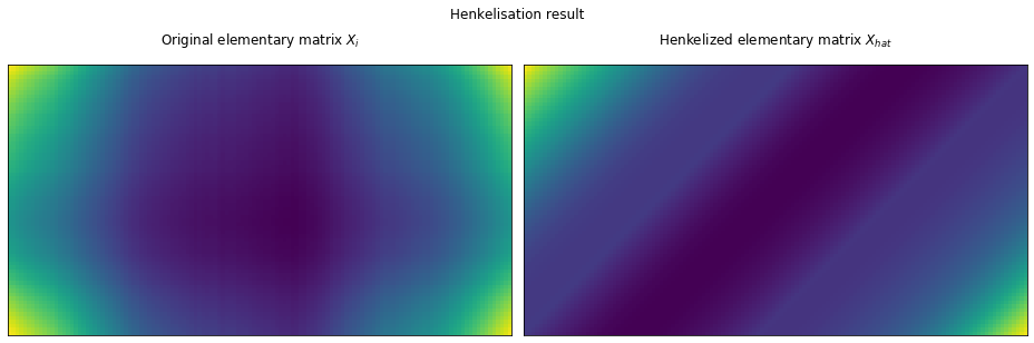
fig, (ax1, ax2) = plt.subplots(1, 2, figsize=(13, 5))
ax1, ax2 = no_axis(ax1), no_axis(ax2)

ax1.matshow(X_[0])
ax1.set_title(r"Original elementary matrix $X_i$")

ax2.matshow(henkelize(X_[0]))
ax2.set_title(r"Henkelized elementary matrix $X_{hat}$")
fig.suptitle("Henkelisation result")
fig.tight_layout();

Quoting the original source,

it is important to note that $\hat{\mathcal{H}}$ is a linear operator, i.e. $\hat{\mathcal{H}}(\mathbf{A} + \mathbf{B}) = \hat{\mathcal{H}}\mathbf{A} + \hat{\mathcal{H}}\mathbf{B}$. Then, for a trajectory matrix $\mathbf{X}$, \(\begin{align*} \hat{\mathcal{H}}\mathbf{X} & = \hat{\mathcal{H}} \left( \sum_{i=0}^{d-1} \mathbf{X}_i \right) \\ & = \sum_{i=0}^{d-1} \hat{\mathcal{H}} \mathbf{X}_i \\ & \equiv \sum_{i=0}^{d-1} \tilde{\mathbf{X}_i} \end{align*}\) As $\mathbf{X}$ is already a Hankel matrix, then by definition $\hat{\mathcal{H}}\mathbf{X} = \mathbf{X}$. Therefore, the trajectory matrix can be expressed in terms of its Hankelised elementary matrices: \(\mathbf{X} = \sum_{i=0}^{d-1} \tilde{\mathbf{X}_i}\)

Which means that doing the henkelisation on all the elementary matrices X resulted from the decomposition will not destroy the additive property of the elementary matrices. We will still end up with a set of elementary matrices that add up to the original henkelized X that we started from. Only now, the great benefit of them being the henkel format is that we can extract the time series.

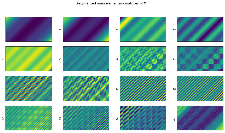
X_hat = np.array([henkelize(X_i) for X_i in _X])

Code

show_elementary_matrices(X_hat, d, max_matices_to_show=15)

Code

from matplotlib import animation, rc
from IPython.display import HTML

def init():
    fig, (ax1, ax2) = plt.subplots(1, 2, figsize=(10, 5))
    ax1, ax2 = no_axis(ax1), no_axis(ax2)

    plot = ax1.matshow(np.sum(X_hat[:d], axis=0))
    ax1.set_title(f"Partial reconstruction using only first {1} components")

    ax2.matshow(X)
    ax2.set_title("Original matrix")

    fig.tight_layout()
    return fig, ax1, plot

def animate(i, plot):
    ax1.set_title(f"Recon. with {i} comp.")
    plot.set_data(np.sum(X_hat[:i], axis=0))
    return [plot]

fig, ax1, plot = init()
anim = animation.FuncAnimation(fig, animate, fargs=(plot,), frames=min(d, 100), interval=100, blit=False)
display(HTML(anim.to_html5_video()))
plt.close()

Code

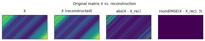
plot_original_vs_rec(X, X_hat)

Extracting the elementary timeseries

So now, let’s just extract the time series components from each of the henkelized elementary matricies.

def timeseries(X_):
    return np.concatenate((X_[0, :], X_[1:, -1]))

[plt.plot(timeseries(X_h)) for X_h in X_hat[:10]]
plt.legend([f"X_hat[{i}]" for i in range(10)], loc=(1.05,0.1));

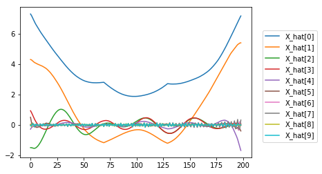
Visually we can assume that:

\[\begin{align*} \tilde{\mathbf{X}}^{\text{(trend)}} & = \tilde{\mathbf{X}}_0 + \tilde{\mathbf{X}}_1 & \implies & \tilde{F}^{\text{(trend)}} = \tilde{F}_0 + \tilde{F}_1 \\ \tilde{\mathbf{X}}^{\text{(periodic 1)}} & = \tilde{\mathbf{X}}_2 + \tilde{\mathbf{X}}_3 & \implies & \tilde{F}^{\text{(periodic 1)}} = \tilde{F}_2 + \tilde{F}_3 \\ \tilde{\mathbf{X}}^{\text{(periodic 2)}} & = \tilde{\mathbf{X}}_4 + \tilde{\mathbf{X}}_5 & \implies & \tilde{F}^{\text{(periodic 2)}} = \tilde{F}_4 + \tilde{F}_5\\ \tilde{\mathbf{X}}^{\text{(noise)}} & = \tilde{\mathbf{X}}_6 + \tilde{\mathbf{X}}_7 + \ldots + \tilde{\mathbf{X}}_{69} & \implies & \tilde{F}^{\text{(noise)}} = \tilde{F}_6 + \tilde{F}_7 + \ldots + \tilde{F}_{69} \end{align*}\]

Code

fig, (ax1, ax2) = plt.subplots(1, 2, figsize=(10, 5))

ax1.plot(timeseries(X_hat[0])+timeseries(X_hat[1]))
ax1.plot(timeseries(X_hat[2])+timeseries(X_hat[3]))
ax1.plot(timeseries(X_hat[4])+timeseries(X_hat[5]))
ax1.plot(np.sum([timeseries(X_hat[i]) for i in range(6, d)], axis=0), alpha=0.2)
ax1.legend(["Trend", "Seasionality_1", "Seasionality_2", "Noise"], loc=(0.025,0.74))
ax1.set_title("Reconstructed components")

ax2.plot(apply(trend, T), alpha=0.4)
ax2.plot(apply(period_1, T), alpha=0.4)
ax2.plot(apply(period_2, T), alpha=0.4)
ax2.plot(apply(noise, T), alpha=0.4)
ax2.legend(["trend", "period_1", "period_2", "noise", "function"], loc='upper right')
ax2.set_title("Original components");

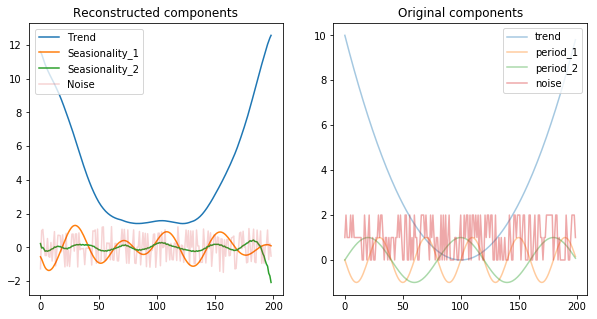
There are a few observations we can draw from the above image:

• The components are scaled / normalized (noise was in the range 0 and 2 originally, while the reconstructions puts it in the range -1 and 1)
• We’re still left with some seasionality component into the noise, evidenced by the wiggly shape of it and by the fact that the second seasionality component has a lower amplitude than we’ve expected
• The first seasinoality component was not actually decomposed entierly. It seems that it is actually a composition of two shapes, in this case each from the other original seasionality element. This is evidenced by the uneven ampltides in it (which usually happens when you add up regular waves with different amplitudes and frequencies).

The kaggle kernel we’ve kept refencing offers a quicker way of extracting the timeseries directly from the elementary matrices $X_i$ (bypassing the henkelisation steps). Let’s compare our extractinos with theirs both visually and quantitavely.

def timeseries_from_elementary_matrix(X_i):
    """Averages the anti-diagonals of the given elementary matrix, X_i, and returns a time series."""
    # Reverse the column ordering of X_i
    X_rev = X_i[::-1]
    # Full credit to Mark Tolonen at https://stackoverflow.com/a/6313414 for this one:
    return np.array([X_rev.diagonal(i).mean() for i in range(-X_i.shape[0]+1, X_i.shape[1])])

Code

fig, (ax1, ax2, ax3) = plt.subplots(1, 3, figsize=(15, 5))

ax1.plot(timeseries(X_hat[0])+timeseries(X_hat[1]))
ax1.plot(timeseries(X_hat[2])+timeseries(X_hat[3]))
ax1.plot(timeseries(X_hat[4])+timeseries(X_hat[5]))
ax1.plot(np.sum([timeseries(X_hat[i]) for i in range(6, d)], axis=0), alpha=0.2)
ax1.legend(["Trend", "Seasionality_1", "Seasionality_2", "Noise"], loc=(0.025,0.74))
ax1.set_title("Step-by-step reconstruction")

ax2.plot(timeseries_from_elementary_matrix(X_[0])+timeseries_from_elementary_matrix(X_[1]))
ax2.plot(timeseries_from_elementary_matrix(X_[2])+timeseries_from_elementary_matrix(X_[3]))
ax2.plot(timeseries_from_elementary_matrix(X_[4])+timeseries_from_elementary_matrix(X_[5]))
ax2.plot(np.sum([timeseries_from_elementary_matrix(X_[i]) for i in range(6, d)], axis=0), alpha=0.2)
ax2.legend(["Trend", "Seasionality_1", "Seasionality_2", "Noise"], loc=(0.025,0.74))
ax2.set_title("Direct reconstruction")

ax3.plot(apply(trend, T), alpha=0.4)
ax3.plot(apply(period_1, T), alpha=0.4)
ax3.plot(apply(period_2, T), alpha=0.4)
ax3.plot(apply(noise, T), alpha=0.4)
ax3.legend(["trend", "period_1", "period_2", "noise", "function"], loc='upper right')
ax3.set_title("Original components");

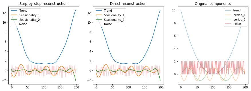
Testing that we get the same reconstructed values from both methods.

for i in range(d):
    assert np.allclose(timeseries(X_hat[i]), timeseries_from_elementary_matrix(X_[i]))

Yup, the same values!

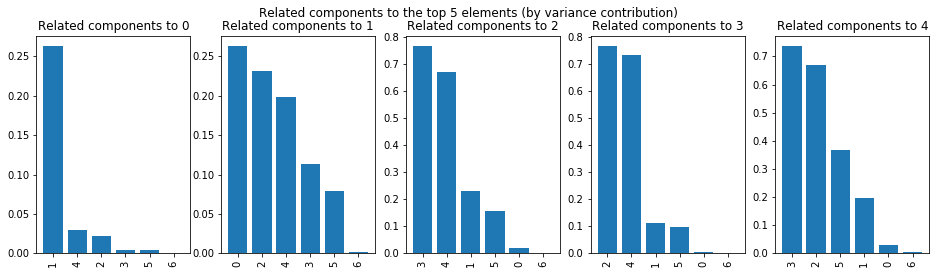
Step 3: Grouping

Obviously grouping in such a manner as we did above (visually) is both error-prone and time consuming and we need a more automated / structured way of doing this. The kaggle kernel we’ve kept refencing offers one such approach.

It’s based on the idea of:

• computing a similariy metric between each timeseries component extracted.
• use the resulted similarity matrix on deciding a way to group (still by manual inspection).

components = np.array([timeseries(X_h) for X_h in X_hat])
last_relevant = relevant_elements(S, variance=0.97)[-1]

Code

def show_top_correlations(ax, component, top=10, variance=0.96):
    last_relevant = relevant_elements(S, variance=variance)[-1]
    top = min(top, last_relevant + 1)
    most_correlated = np.argsort(Wcorr[component, :top])[::-1][1:]
    ax.bar(np.arange(1, top), Wcorr[component, most_correlated])
    ax.set_xticks(np.arange(1, top))
    ax.set_xticklabels(most_correlated[:top])
    ax.tick_params(axis='x', rotation=90)
    ax.set_title(f"Related components to {component}")
    
    
fig, (ax1, ax2, ax3, ax4, ax5) = plt.subplots(1, 5, figsize=(16, 4))
show_top_correlations(ax1, 0, 10)
show_top_correlations(ax2, 1, 10)
show_top_correlations(ax3, 2, 10)
show_top_correlations(ax4, 3, 10)
show_top_correlations(ax5, 4, 10)
fig.suptitle("Related components to the top 5 elements (by variance contribution)");

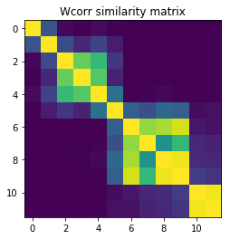
Computing a similarity matrix

We’re going to explore multiple ways of comparing the timeseries components and choose one that seems more promissing.

Similarity method 1: Weighted dot product

The kernel uses a weighted, normalized dot product of two vectors as the similarity matrix.

For two reconstructed time series, \(\tilde{F}_i\) and \(\tilde{F}_j\), of length $N$, and a window length $L$, we define the weighted inner product, \((\tilde{F}_i, \tilde{F}_j)_w\) as: \((\tilde{F}_i, \tilde{F}_j)_w = \sum_{k=0}^{N-1} w_k \tilde{f}_{i,k} \tilde{f}_{j,k}\) where \(\tilde{f}_{i,k}\) and \(\tilde{f}_{j,k}\) are the $k$th values of \(\tilde{F}_i\) and \(\tilde{F}_j\), respectively

Put simply, if \((\tilde{F}_i, \tilde{F}_j)_w = 0\), \(\tilde{F}_i\) and \(\tilde{F}_j\) are w-orthogonal and the time series components are separable. Of course, total w-orthogonality does not occur in real life, so instead we define a \(d \times d\) weighted correlation matrix, \(\mathbf{W}_{\text{corr}}\), which measures the deviation of the components $\tilde{F}_i$ and \(\tilde{F}_j\) from w-orthogonality. The elements of \(\mathbf{W}_{\text{corr}}\) are given by

\[W_{i,j} = \frac{(\tilde{F}_i, \tilde{F}_j)_w}{\lVert \tilde{F}_i \rVert_w \lVert \tilde{F}_j \rVert_w}\]

where \(\lVert \tilde{F}_k \rVert_w = \sqrt{(\tilde{F}_k, \tilde{F}_k)_w}\) for $k = i,j$.

The interpretation of \(W_{i,j}\) is straightforward: if \(\tilde{F}_i\) and \(\tilde{F}_j\) are arbitrarily close together (but not identical), then \((\tilde{F}_i, \tilde{F}_j)_w \rightarrow \lVert \tilde{F}_i \rVert_w \lVert \tilde{F}_j \rVert_w\) and therefore \(W_{i,j} \rightarrow 1\). Of course, if \(\tilde{F}_i\) and \(\tilde{F}_j\) are w-orthogonal, then \(W_{i,j} = 0\). Moderate values of \(W_{i,j}\) between 0 and 1, say \(W_{i,j} \ge 0.3\), indicate components that may need to be grouped together.

The similarity metric looks awfully similar to a cosine similarity between two vectors, only that this time the inner product is weighted by the dimension of each antidiagonal (so by how many times each value in $x_i, x_j$ appears in their own henkelized matrix).

It’s important to note here that both $x_i$ and $x_j$ are values found at the same index (position) in theis respective timeseries component $F_i$ and $F_j$. It’s because of this, that they have an equal weight (i.e. their multiplier in the henkelized matrix is given by the dimension of the antidiagonal that owns them, which is has the same value, because they share the same position).

Let’s compute the w array first (the weights).

Code

shape = (5, 10)
a = np.zeros(shape=shape, dtype=np.int)
for i in range(a.shape[0]):
    for j in range(a.shape[1]):
        a[i, j] = len(list(antidiagonal((i, j), shape)))


fig, (ax, ax2) = plt.subplots(2, 1, figsize=(10, 5))
ax = no_axis(ax)

ax.matshow(a, cmap=plt.cm.Blues)

for i in range(a.shape[0]):
    for j in range(a.shape[1]):
        ax.text(j, i, str(a[i, j]), va='center', ha='center')
ax.set_title("Parent antidiagonal dimension owning each element")    


counts = timeseries(a) 
ax2.matshow([counts], cmap=plt.cm.Blues)
ax2.set_xticks(list(range(a.shape[0] + a.shape[1])))
for i in range(a.shape[0] + a.shape[1] - 1):
    ax2.text(i, 0, str(counts[i]))

ax2.get_yaxis().set_visible(False)
ax2.xaxis.tick_bottom()
ax2.set_xlim((-0.5, a.shape[0] + a.shape[1] - 1.5))
ax2.set_title("Unrolled dimension of antidiagonal containing each element (the W array)");

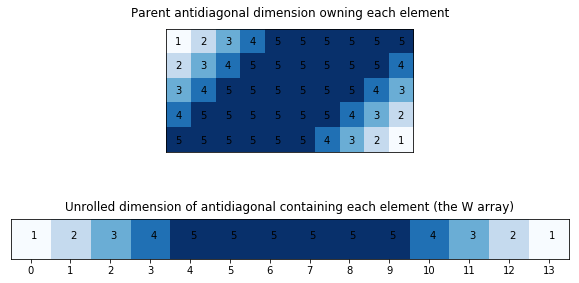
def compute_weights_array(L, N_K):
    return np.array(list(np.arange(L)+1) + [L ]*(N-L-1) + list(np.arange(L)+1)[::-1])

w = compute_weights_array(5, 10)
w

array([1, 2, 3, 4, 5, 5, 5, 5, 5, 5, 4, 3, 2, 1])

We’re going to compute the $W_{corr}$ matrix and only retain the elements that ensure 97% of the variance.

w = compute_weights_array(70, 200 - 70)

# Calculate the individual weighted norms, ||F_i||_w, first, then take inverse square-root so we don't have to later.
F_wnorms = np.array([w.dot(components[i]**2) for i in range(d)])
F_wnorms = F_wnorms**-0.5

# Calculate the w-corr matrix. The diagonal elements are equal to 1, so we can start with an identity matrix
# and iterate over all pairs of i's and j's (i != j), noting that Wij = Wji.
Wcorr = np.identity(d)
for i in range(d):
    for j in range(i+1,d):
        Wcorr[i,j] = abs(w.dot(components[i]*components[j]) * F_wnorms[i] * F_wnorms[j])
        Wcorr[j,i] = Wcorr[i,j]
        
plt.imshow(
    Wcorr[:last_relevant, :last_relevant],
    vmin=0,
    vmax=1
)
plt.title("Wcorr similarity matrix");

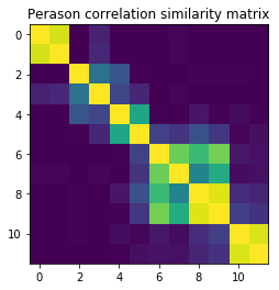
Similarity method 2: Covariance matrix

Given that the above is a weighted correlation measurement, and since the weights basically don’t do much beside penalizing the edge values (a bit) we could approximate the computation by using a plaint Perason correlation.

Sure we won’t have the edges penalized anymore but the series is a long one anyway, compared to the window size, so the vast majority of values will have an equal weight.

If this works reasonalby well (the results look somewhat similar) we could get away with fewer code and a cleaner architecture.

Corr_perason = np.corrcoef(components)
Corr_perason[Corr_perason < 0] = 0
plt.imshow(
    Corr_perason[:last_relevant, :last_relevant],
    vmin=0,
    vmax=1
)
plt.title("Perason correlation similarity matrix");

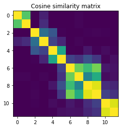
Similarity method 3: Cosine similarity

Since we’ve noted before that

The similarity metric looks awfully similar to a cosine similarity between two vectors, only that this time the inner product is weighted by the dimension of each antidiagonal (so by how many times each value in $x_i, x_j$ appears in their own henkelized matrix).

we’ll try that as well to see how it behaves.

from sklearn.metrics.pairwise import cosine_similarity
cos_sim = cosine_similarity(components)
cos_sim[cos_sim < 0] = 0
plt.imshow(
    cos_sim[:last_relevant, :last_relevant],
    vmin=0,
    vmax=1
)
plt.title("Cosine similarity matrix");

Comparing the metrics and choosing one

Code

def _diff(sim1, sim2):
    return np.round(np.power(sim1[:last_relevant, :last_relevant] - sim2[:last_relevant, :last_relevant], 2), 3)

fig, (ax1, ax2, ax3) = plt.subplots(1, 3, figsize=(15, 5))
ax1, ax2, ax3 = no_axis(ax1), no_axis(ax2), no_axis(ax3)

ax1.imshow(
    _diff(Wcorr, Corr_perason),
    vmin=0,
    vmax=1
)
ax1.set_title(r"$|Wcorr - Corr\_pearson|^2$")

ax2.imshow(
    _diff(Wcorr, cos_sim),
    vmin=0,
    vmax=1    
)
ax2.set_title(r"$|Wcorr - cos\_sim|^2$")

ax3.imshow(
    _diff(cos_sim, Corr_perason),
    vmin=0,
    vmax=1
)
ax3.set_title(r"$|cos\_sim - Corr\_pearson|^2$")

fig.suptitle("Comparision between the three similarity metrics");

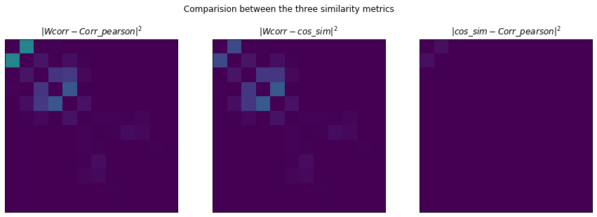
Plotting the distance between each similarity method pair we can see that:

• Perason correlation and cosine similarity yield very similar results
• Pearson correlation seem the better capture the correlation between the first two components (so is better in this respect to the cosine similarity)
  • The main difference is between components 0 and 1. On the Pearson correlation, the similarity between them is really strong, while on the custom similarity there isn’t nearly as much similarity. Since 0 and 1 by visual inspection should be grouped togheter it seems a better performer would be the Perason correlation (at least on this example).
• The weighted correalation is stronger on the second group (2, 3, 4) than the other two.

It’s thus a tough call but due to the simpler code the Perason correlation might give the best tradeoffs.

Clustering the components using the similarity matrix

Next we will cluster the elements using the similarity matrix and AffinityPropagation.

from sklearn.cluster import AffinityPropagation

similarity_matrix = Corr_perason
last_relevant = relevant_elements(S, variance=0.96)[-1]
relevant_block_matrix = similarity_matrix[:last_relevant+1, :last_relevant+1]
clusters = AffinityPropagation(affinity='precomputed').fit_predict(relevant_block_matrix)
clusters

array([0, 0, 1, 1, 2, 2, 2])

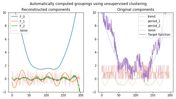
Results

Ok, we’ve come this far, and… let’s see what we’ve got!

Code

# Plotting of the clusters
fig, (ax1, ax2) = plt.subplots(1, 2, figsize=(10, 5))

unique_clusters = sorted(np.unique(clusters))
for cluster in unique_clusters:
    series = np.array([timeseries(X_hat[i]) for i in np.where(clusters == cluster)[0]])
    ax1.plot(series.sum(axis=0))

ax1.plot(np.sum([timeseries(X_hat[i]) for i in range(last_relevant+1, d)], axis=0), alpha=0.2)
ax1.legend([f"F_{i}" for i in unique_clusters] + ["noise"], loc=(0.025,0.74))
ax1.set_title("Reconstructed components")
ax1.set_ylim(-2, 10)

ax2.plot(apply(trend, T), alpha=0.3)
ax2.plot(apply(period_1, T), alpha=0.3)
ax2.plot(apply(period_2, T), alpha=0.3)
ax2.plot(apply(noise, T), alpha=0.3)
plt.plot(apply(f, T), alpha=0.9)
ax2.legend(["trend", "period_1", "period_2", "noise", "Target function"], loc='upper right')
ax2.set_title("Original components")
ax2.set_ylim(-2, 10)
fig.suptitle("Automatically computed groupings using unsupervised clustering");

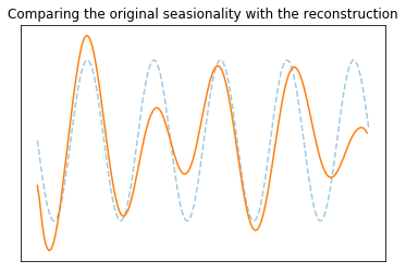
Comparing the seasonality of the reconstruction and the original seasionality (2)

Code

plt.plot(apply(period_1, T), "--", alpha=0.4)
series = np.array([timeseries(X_hat[i]) for i in np.where(clusters == 1)[0]])
plt.plot(series.sum(axis=0))
plt.title("Comparing the original seasionality with the reconstruction")
plt.xticks([]); plt.yticks([]);

Conclusions

SSA seems to be a powerfull technique! We were able to reconstruct a large part of the components. Overall we’d like to point out the following:

• when the noise is to strong (like in our case) not all components can be reconstructed
• SSA (as descibed here):
  • works on timeseries data
  • relies on transforming it into a 2D (trajectory) matrix
  • is using SVD on the trajectory matrix to decopose it into a sum of elementary matrices
  • forces the elementary matrices into henkel form via diagonal averaging (which preserves the addition property)
  • extracts the timeseries components from the diagonalized elementary matrices
• a grouping of the timeseries components is necessary to reconstruct the original components
• the grouping is based on defining a good similarity metric between components, possible metrics being:
  • anti-diagonal weighed correlation
  • Perason correlation
  • cosine similarity
• in our case, Person correlation proved to be both performant and less verbose
• clustering can be used to automatically group the elementary components (via the similarity matirx).
• hyperparameters that need to be choosen well:
  • L - the window length when building the trajectory matrix
    • start with larger values (max is N/2) and decrease until a suitable result
  • variance we need to retain before grouping (similar to setting the noise threshold). Retaining a higher variance (e.g. 99%) leads to many elementary components (with a low contribution) to be included in the clustering, leading to more grouped components than necessary

Based on:

1. Wikipedia article
2. Kaggle kernel