Mean Shift

Mean Shift Clustering

The algorithm was proposed by Dorin Comaniciu (a fellow romanian) here.

Idea of mean-shift

Core: Mean-shift replaces all the values with their weighted averages of distance to the all the other points.

• So for each point we must compute the distances to all the other points
• Do a weighted mean (large distances should be multiplied by low weights, and viceversa) - using the gaussian kernel.
• Replace the starting point with the resulting mean.
• Repeat until convergence.

Define a set of clusters

def generate_clusters(n_clusters, n_samples, noise_level=0.08, scale=8):
    """
    Returns N center points and (N,S) sample points that have a noise ratio of NL.
    
    The points will be scaled to with the given value
    """
    centroids = np.random.randn(n_clusters, 2)
    clusters = np.random.randn(n_clusters, n_samples, 2) * noise_level + np.expand_dims(centroids, axis=1)
    return centroids*scale, clusters*scale

def plot_clusters(centroids, clusters):
    """
    Print a chart with the centroids and clusters in different colors
    """
    colors = (list('bgrcmykw')*3)
    for i in range(len(centroids)):
        plt.scatter(clusters[i, :, 0], clusters[i, :, 1], c=colors[i])
    plt.scatter(centroids[:, 0], centroids[:, 1], c='red', marker='x')
    
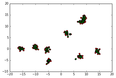
centroids, clusters = generate_clusters(9, 20)
plot_clusters(centroids, clusters)

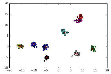
We know the clusters that we generated but we want to forget the grouping. We reshape the clusters into a single large array that contains nD (in this case 2D) points.

all_points = clusters.reshape(clusters.shape[0]*clusters.shape[1], -1)
print(all_points.shape)

(180, 2)

Weights kernel

Kernel - When you define a curve whose results all add (the integral of it) up to 1

The probability density function of a normally distributed random variable with expected value μ (mean) and variance $σ^2$ is given by the bellow gaussian function:

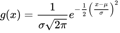
Because it’s a probability distribution, the sum (integral) of this function is 1, this by the definition above is a gaussian kernel

If we have a μ = 0 then we have the simplifyed gaussian, g(x, σ) as follows:

from math import pi
def gaussian(x, std): 
    return np.exp(-0.5*((x/std)**2)) / (std * np.sqrt(2*pi))

Note: Because we assumed μ = 0 it’s really important to normalize all the features before trying to cluster!

Plots of the gaussian function

Plot the above gaussian formula

import numpy as np
def random_sample(size):
    """
    Returns size numbers between -5 and 5 in a np.array
    """
    return (np.random.sample(size) - 0.5) * 10
random_sample(10)

array([ 0.29430649, -2.84212033,  2.09673585, -2.50085473, -0.13159073,
        0.28121437,  4.59805783,  3.93600877,  3.31028357, -0.8424589 ])

from matplotlib import pyplot as plt

x = random_sample(100) 
plt.scatter(x, gaussian(x, 1))

<matplotlib.collections.PathCollection at 0x7f4e5e0e8b50>

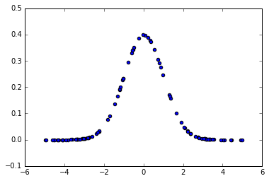
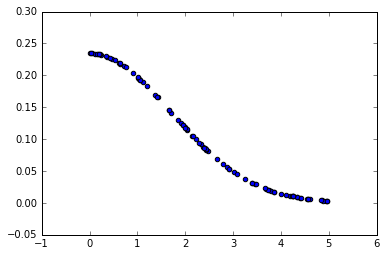
We are interested only on the >0 half of the gaussian because we will use it as a continous weighting function. When a x is close to 0 (i.e. a distance between two close points) we will want to assign a large weight to it, and inversly, when x is large, we want a really small weight.

The std parameter defines how fast/slow the weights go to 0 when x increases (similar to a velocity factor)

x = random_sample(200) 
x = x[x >= 0]

std = 1.7
plt.scatter(x, gaussian(x, std))

Step by step implementation

So, first we compute the euclidian distance from one point to every other point.
We do this on each of the dimensions individually and then add the distances together into a single value.

Basically we do $dist_i(x,y) = \sqrt{(x - x_i)^2 + (y - y_i)^2}$

We end up with as many distances are there are points.

point = all_points[0]
all_distances = np.sqrt((point - all_points) ** 2).sum(axis=1)
all_distances.shape

(180,)

Then we need to compute the weights for all the distances using the kernel of our choosing (in this case the gaussian kernel above).
We should be left with as many weights as we have distances.

weights = gaussian(all_distances, 1.7)
weights.shape

(180,)

We then multiply the coordinates (second axis) of each point with their corresponding weight. This magnifies their contribution to the final value for coordinate position, if the point is close to our target (To anticipate, we will aggregate all the values of each coordinate on all points by averageing them all up).

Note: Because each weight is scalar now, and we need to apply them on all features, we need to expand to (nr, 1) dimensionality in order for the broadcasting in numpy to apply it on all the values of the second axis.

(all_points * np.expand_dims(weights, 1)).shape

(180, 2)

We then do a weighted average of the points and weights. We’re saying that we want to move towards each point but using the weight as the acceleration parameter.

$(x, y) = (\frac{\sum_{i=1}^{n}{x_i*weight_i}}{\sum_{i=1}^{n}{weight_i}}, \frac{\sum_{i=1}^{n}{y_i*weight_i}}{\sum_{i=1}^{n}{weight_i}})$

The final result (the new x) should be a point as well, n-dimensional.

new_x = (all_points * np.expand_dims(weights, 1)).sum(axis=0) / weights.sum()
new_x.shape

(2,)

Full implementation

def mean_shift_update(all_points, std=0.5):
    X = np.copy(all_points)
    for i, point in enumerate(all_points):
        distances = np.sqrt(((point - all_points) ** 2).sum(axis=1))
        weights = gaussian(distances, std)
        X[i] = (np.expand_dims(weights, 1) * all_points).sum(axis=0) / weights.sum()
    return X

def mean_shift(X, std=2.5, iterations=10):
    X = np.copy(X)
    for i in range(iterations):
        X = mean_shift_update(X)
    return X

Analisys

We will print a single iteration of the algorithm. In red we have the initial dots, while in green we have the updates. It’s clear from this that all the points move towards the cluster center.

update = all_points
plt.scatter(update[:, 0], update[:, 1], c='red')
update = mean_shift_update(update)
plt.scatter(update[:, 0], update[:, 1], c='green')

Std and iteration discussions

The std paramter has been an enigma until now. We need to see how it affects the overal performance.

First, we add some utilitary code that we use to generate animations of the mean_shift_update routine.

from matplotlib import animation, rc
from IPython.display import HTML

data = None

# animation function. This is called sequentially
def animate(i, scatt, std):
    global data
    scatt.set_offsets(data)
    data = mean_shift_update(data, std)
    return (scatt,)

def show_mean_shift(std, iterations, speed):
    global data
    data = np.copy(all_points)
    fig = plt.figure()

    scatt = plt.scatter(data[:, 0], data[:, 1])
    plt.close()
    
    anim = animation.FuncAnimation(fig, animate, fargs=(scatt,std), frames=iterations, interval=speed, blit=False)
    return HTML(anim.to_html5_video())

First, how is the algotithm working with .5 std?

show_mean_shift(.5, 10, 150)

With std=2 we see that some of the clusters are merged into a single one, so choosing the std well is key to efficient mean shift usage.

show_mean_shift(2, 10, 150)

On std=5 we clearly see the impact of it. This setting merges everything together into a cuple large clusters.

show_mean_shift(5, 10, 150)

Choosing a best std (or bandwith as is called in the mean-shift algorithm) isn’t that straight forward. It really depends on the data at hand (of the type of problem you need to solve).

There are some ways of doing this but are hidden in research papers under piles of greek symbols.

The easiest way of doing this is by using the estimate_bandwith function from scikit-learn. But as you’ll see bellow it doesn’t yield good results.

In our case the implementation is incompatible with this function (as shown when we discuss the Scikit-learn implementation further).

from sklearn.cluster import estimate_bandwidth
estimate_bandwidth(all_points)

9.2146098764578248

show_mean_shift(estimate_bandwidth(all_points), 5, 300)

Iteration discussion

Another aspect that usually influences the final result is the number of iterations that you use. Let’s thake the example we gave for std=2. Remeber that we used 10 iterations and the result was like the one bellow.

show_mean_shift(2, 10, 120)

Now notice what happens if we let the algoritm run for four times as many iterations.

show_mean_shift(2, 40, 120)

We initially thought the 6 cluster solution was the convergence point, but if we let it run more we see that two aditional clusters are merged into a single one.

You should thus be very carefull when choosing both the std and iteration number when using mean-shift.

“Early stopping” might be a good solution for automatically selecting the iteration limit, but this is again really specific to the problem domain.

Scikit-learn implementation

You can find a better implementation of mean-shift in sklearn under sklearn.cluster.MeanShift. It differs from this in that it uses KNN to select a subset of good candidate points and then directly computes the mean point from those (skipping the gaussian kernel altogheter). By doing this we also solve the iteration instability case above because the two clusters that merge in the end won’t be in the other’s vicinity so will not contribute to each other’s means.

The bandwith parameter, computed by estimate_bandwith function actually defines the radius used by KNN for candidate selection.

This explains why this function cannot be used in computing the std on our own version.

from sklearn.cluster import MeanShift

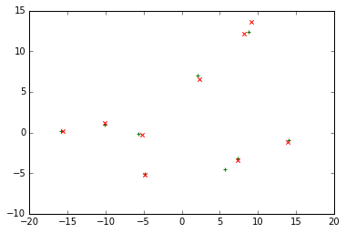
Empirical results show that 1.18 yields much of the same results as std=0.5 in our implementation. The centroids thus found are pretty much the same with ours.

ms = MeanShift(bandwidth=1.18)
ms.fit(all_points)

centroids_found = ms.cluster_centers_
plt.scatter(centroids_found[:, 0], centroids_found[:, 1], c='g', marker='+')
plt.scatter(centroids[:, 0], centroids[:, 1], c='r', marker='x')

The MeanShift version also impements the “early stopping” strategy by using the follwing metric:

• on each point, after computing the new value (the mean of it’s neighbours) compare by what distance did it move
• if it moved less than stop_threshold then stop trying.

stop_threshold is 0.001*bandwidth

Conclusion

Mean-Shift is a good clustering method, but has some limitations in that you need to know the correct values for the bandwith and the number of iterations until convergence.

We’ve showed what bandwith actually is in the original paper and how, in sklearn this term defines a completely different concept.

Overall, sklearn implements a more robust (I would argue) version, a simpler one and also one that runs faster (in O(T*n*log(n) rather than O(T*n^2)). It also has a nice estimate_bandwith function that, if you’re lucky and the data you work on is suited to it, will automatically find a good bandwith paramter for you.