
Beating mnist
Summary
Contents
- What is MNIST
- Collection of 70 000 hand written digits
- Gathered by the USPS (United States Post Service)
- Problem description
- Given an image with a hand written digit, corectly identify it
- 0, 1, 2, …, 9
- State of the art is 99.7% accuracy!
- Going from nothing to stat-of-the-art
Beating MNIST
Setup
The machine
- AWS p2.xlarge instance
- CUDA K80 GPU
- Costs 1$/hour so let’s be quick!
!nvidia-smi
Wed Jul  5 15:38:31 2017
+-----------------------------------------------------------------------------+
| NVIDIA-SMI 375.39                 Driver Version: 375.39                    |
|-------------------------------+----------------------+----------------------+
| GPU  Name        Persistence-M| Bus-Id        Disp.A | Volatile Uncorr. ECC |
| Fan  Temp  Perf  Pwr:Usage/Cap|         Memory-Usage | GPU-Util  Compute M. |
|===============================+======================+======================|
|   0  Tesla K80           Off  | 0000:00:1E.0     Off |                    0 |
| N/A   42C    P0    55W / 149W |    118MiB / 11439MiB |      0%      Default |
+-------------------------------+----------------------+----------------------+

+-----------------------------------------------------------------------------+
| Processes:                                                       GPU Memory |
|  GPU       PID  Type  Process name                               Usage      |
|=============================================================================|
|    0     25353    C   /home/ubuntu/anaconda2/bin/python              116MiB |
+-----------------------------------------------------------------------------+
Basic setup
Load some utilitaries, nothing fancy
%matplotlib inline
import numpy as np

import utils; reload(utils)
from utils import plots
from matplotlib import pyplot as plt
Using Theano backend.
Using gpu device 0: Tesla K80 (CNMeM is disabled, cuDNN 5103)
/home/ubuntu/anaconda2/lib/python2.7/site-packages/theano/sandbox/cuda/__init__.py:600: UserWarning: Your cuDNN version is more recent than the one Theano officially supports. If you see any problems, try updating Theano or downgrading cuDNN to version 5.
  warnings.warn(warn)
Download the MNIST dataset
from keras.datasets import mnist
(x_train, y_train), (x_test, y_test) = mnist.load_data()
y_train.shape, y_test.shape
((60000,), (10000,))
x_train.shape
(60000, 28, 28)
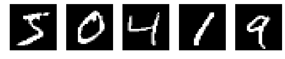
Print some of the data
# Data shape
print(x_train.shape)
# show raw pixels
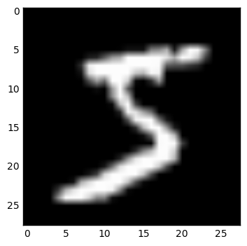
plt.imshow(x_train[0], cmap='gray')
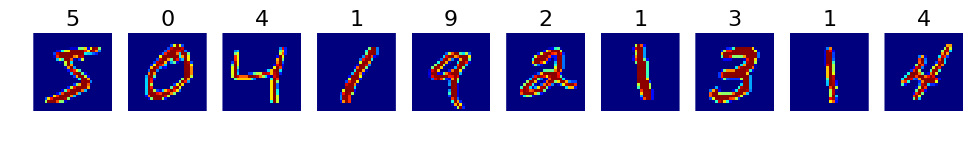
# plot the first 10 images
plots(x_train[:10], titles=y_train[:10])
(60000, 28, 28)
Data massaging
Expand dimension with color channel.
The images in the dataset are bitmap-like images but we need images that have at least one color channel.
X = np.expand_dims(x_train, 1)
print(X.shape)

X_val = np.expand_dims(x_test, 1)
(60000, 1, 28, 28)
x_train[10]
array([[  0,   0,   0,   0,   0,   0,   0,   0,   0,   0,   0,   0,   0,   0,   0,   0,   0,   0,
          0,   0,   0,   0,   0,   0,   0,   0,   0,   0],
       [  0,   0,   0,   0,   0,   0,   0,   0,   0,   0,   0,   0,   0,   0,   0,   0,   0,   0,
          0,   0,   0,   0,   0,   0,   0,   0,   0,   0],
       [  0,   0,   0,   0,   0,   0,   0,   0,   0,   0,   0,   0,   0,   0,   0,   0,   0,   0,
          0,   0,   0,   0,   0,   0,   0,   0,   0,   0],
       [  0,   0,   0,   0,   0,   0,   0,   0,   0,   0,   0,   0,   0,   0,   0,   0,   0,   0,
          0,   0,   0,   0,   0,   0,   0,   0,   0,   0],
       [  0,   0,   0,   0,   0,   0,   0,   0,   0,   0,   0,  42, 118, 219, 166, 118, 118,   6,
          0,   0,   0,   0,   0,   0,   0,   0,   0,   0],
       [  0,   0,   0,   0,   0,   0,   0,   0,   0,   0, 103, 242, 254, 254, 254, 254, 254,  66,
          0,   0,   0,   0,   0,   0,   0,   0,   0,   0],
       [  0,   0,   0,   0,   0,   0,   0,   0,   0,   0,  18, 232, 254, 254, 254, 254, 254, 238,
         70,   0,   0,   0,   0,   0,   0,   0,   0,   0],
       [  0,   0,   0,   0,   0,   0,   0,   0,   0,   0,   0, 104, 244, 254, 224, 254, 254, 254,
        141,   0,   0,   0,   0,   0,   0,   0,   0,   0],
       [  0,   0,   0,   0,   0,   0,   0,   0,   0,   0,   0,   0, 207, 254, 210, 254, 254, 254,
         34,   0,   0,   0,   0,   0,   0,   0,   0,   0],
       [  0,   0,   0,   0,   0,   0,   0,   0,   0,   0,   0,   0,  84, 206, 254, 254, 254, 254,
         41,   0,   0,   0,   0,   0,   0,   0,   0,   0],
       [  0,   0,   0,   0,   0,   0,   0,   0,   0,   0,   0,   0,   0,  24, 209, 254, 254, 254,
        171,   0,   0,   0,   0,   0,   0,   0,   0,   0],
       [  0,   0,   0,   0,   0,   0,   0,   0,   0,   0,   0,   0,  91, 137, 253, 254, 254, 254,
        112,   0,   0,   0,   0,   0,   0,   0,   0,   0],
       [  0,   0,   0,   0,   0,   0,   0,   0,   0,   0,  40, 214, 250, 254, 254, 254, 254, 254,
         34,   0,   0,   0,   0,   0,   0,   0,   0,   0],
       [  0,   0,   0,   0,   0,   0,   0,   0,   0,   0,  81, 247, 254, 254, 254, 254, 254, 254,
        146,   0,   0,   0,   0,   0,   0,   0,   0,   0],
       [  0,   0,   0,   0,   0,   0,   0,   0,   0,   0,   0, 110, 246, 254, 254, 254, 254, 254,
        171,   0,   0,   0,   0,   0,   0,   0,   0,   0],
       [  0,   0,   0,   0,   0,   0,   0,   0,   0,   0,   0,   0,  73,  89,  89,  93, 240, 254,
        171,   0,   0,   0,   0,   0,   0,   0,   0,   0],
       [  0,   0,   0,   0,   0,   0,   0,   0,   0,   0,   0,   0,   0,   0,   0,   1, 128, 254,
        219,  31,   0,   0,   0,   0,   0,   0,   0,   0],
       [  0,   0,   0,   0,   0,   0,   0,   0,   0,   0,   0,   0,   0,   0,   0,   7, 254, 254,
        214,  28,   0,   0,   0,   0,   0,   0,   0,   0],
       [  0,   0,   0,   0,   0,   0,   0,   0,   0,   0,   0,   0,   0,   0,   0, 138, 254, 254,
        116,   0,   0,   0,   0,   0,   0,   0,   0,   0],
       [  0,   0,   0,   0,   0,   0,  19, 177,  90,   0,   0,   0,   0,   0,  25, 240, 254, 254,
         34,   0,   0,   0,   0,   0,   0,   0,   0,   0],
       [  0,   0,   0,   0,   0,   0, 164, 254, 215,  63,  36,   0,  51,  89, 206, 254, 254, 139,
          8,   0,   0,   0,   0,   0,   0,   0,   0,   0],
       [  0,   0,   0,   0,   0,   0,  57, 197, 254, 254, 222, 180, 241, 254, 254, 253, 213,  11,
          0,   0,   0,   0,   0,   0,   0,   0,   0,   0],
       [  0,   0,   0,   0,   0,   0,   0, 140, 105, 254, 254, 254, 254, 254, 254, 236,   0,   0,
          0,   0,   0,   0,   0,   0,   0,   0,   0,   0],
       [  0,   0,   0,   0,   0,   0,   0,   0,   7, 117, 117, 165, 254, 254, 239,  50,   0,   0,
          0,   0,   0,   0,   0,   0,   0,   0,   0,   0],
       [  0,   0,   0,   0,   0,   0,   0,   0,   0,   0,   0,   0,   0,   0,   0,   0,   0,   0,
          0,   0,   0,   0,   0,   0,   0,   0,   0,   0],
       [  0,   0,   0,   0,   0,   0,   0,   0,   0,   0,   0,   0,   0,   0,   0,   0,   0,   0,
          0,   0,   0,   0,   0,   0,   0,   0,   0,   0],
       [  0,   0,   0,   0,   0,   0,   0,   0,   0,   0,   0,   0,   0,   0,   0,   0,   0,   0,
          0,   0,   0,   0,   0,   0,   0,   0,   0,   0],
       [  0,   0,   0,   0,   0,   0,   0,   0,   0,   0,   0,   0,   0,   0,   0,   0,   0,   0,
          0,   0,   0,   0,   0,   0,   0,   0,   0,   0]], dtype=uint8)
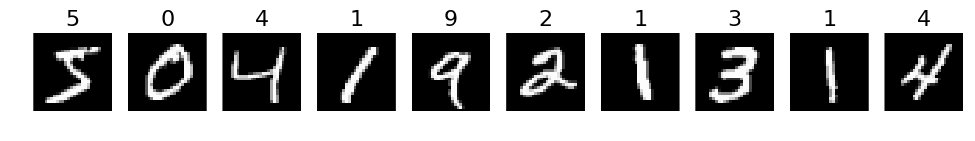
plots(X[:10], titles=y_train[:10])
One-hot-encoding
Method 1 (python code)
Then we need to change the labels to one_hot_encodings
def one_hot_encoded(_y):
    max_class = np.max(_y)
    one_hot = np.zeros((_y.shape[0], max_class+1), dtype=np.float)
    for i, clazz in enumerate(_y):
        one_hot[i][clazz] = 1
    return one_hot

y_ = one_hot_encoded(y_train)
print(y_train[:10])
print(y_[:10])
[5 0 4 1 9 2 1 3 1 4]
[[ 0.  0.  0.  0.  0.  1.  0.  0.  0.  0.]
 [ 1.  0.  0.  0.  0.  0.  0.  0.  0.  0.]
 [ 0.  0.  0.  0.  1.  0.  0.  0.  0.  0.]
 [ 0.  1.  0.  0.  0.  0.  0.  0.  0.  0.]
 [ 0.  0.  0.  0.  0.  0.  0.  0.  0.  1.]
 [ 0.  0.  1.  0.  0.  0.  0.  0.  0.  0.]
 [ 0.  1.  0.  0.  0.  0.  0.  0.  0.  0.]
 [ 0.  0.  0.  1.  0.  0.  0.  0.  0.  0.]
 [ 0.  1.  0.  0.  0.  0.  0.  0.  0.  0.]
 [ 0.  0.  0.  0.  1.  0.  0.  0.  0.  0.]]
Method 2 (keras)
The same effect can be obtain by using the keras function bellow
from keras.utils.np_utils import to_categorical
y = to_categorical(y_train)
y_val = to_categorical(y_test)
Model 1: Linear regression
This is the simplest model possible. We only have one layer, the output one.
from keras.models import Sequential
from keras.layers.core import Lambda

from keras.layers import Dense, InputLayer, Flatten
from keras.optimizers import Adam

model = Sequential([
        Flatten(input_shape=(1, 28, 28)),
        Dense(10, activation='softmax')
    ])

model.compile(optimizer='adam', loss='categorical_crossentropy', metrics=['accuracy'])
model.summary()
____________________________________________________________________________________________________
Layer (type)                     Output Shape          Param #     Connected to
====================================================================================================
flatten_3 (Flatten)              (None, 784)           0           flatten_input_2[0][0]
____________________________________________________________________________________________________
dense_4 (Dense)                  (None, 10)            7850        flatten_3[0][0]
====================================================================================================
Total params: 7850
____________________________________________________________________________________________________
model.fit(X, y, nb_epoch=10, validation_data=(X_val, y_val))
Train on 60000 samples, validate on 10000 samples
Epoch 1/10
60000/60000 [==============================] - 3s - loss: 8.5304 - acc: 0.4673 - val_loss: 7.5085 - val_acc: 0.5318
Epoch 2/10
60000/60000 [==============================] - 3s - loss: 7.3680 - acc: 0.5410 - val_loss: 7.3163 - val_acc: 0.5440
Epoch 3/10
60000/60000 [==============================] - 3s - loss: 7.3185 - acc: 0.5443 - val_loss: 7.4219 - val_acc: 0.5382
Epoch 4/10
60000/60000 [==============================] - 3s - loss: 6.9662 - acc: 0.5663 - val_loss: 6.2782 - val_acc: 0.6084
Epoch 5/10
60000/60000 [==============================] - 3s - loss: 6.0397 - acc: 0.6235 - val_loss: 6.0477 - val_acc: 0.6235
Epoch 6/10
60000/60000 [==============================] - 3s - loss: 5.9435 - acc: 0.6297 - val_loss: 6.2494 - val_acc: 0.6109
Epoch 7/10
60000/60000 [==============================] - 3s - loss: 5.9682 - acc: 0.6283 - val_loss: 6.0403 - val_acc: 0.6235
Epoch 8/10
60000/60000 [==============================] - 3s - loss: 5.9611 - acc: 0.6290 - val_loss: 5.9890 - val_acc: 0.6271
Epoch 9/10
60000/60000 [==============================] - 3s - loss: 5.8919 - acc: 0.6332 - val_loss: 5.9556 - val_acc: 0.6293
Epoch 10/10
60000/60000 [==============================] - 3s - loss: 5.8582 - acc: 0.6351 - val_loss: 6.0442 - val_acc: 0.6244


<keras.callbacks.History at 0x7f7fe297aa50>
We can see that the model is not training that well. It progresses really slowly and the loss is even jumping up and down. This is a sign that the input is data is skewed:
- lower the learning rate (training even slower)
- normalize the inputs
model.optimizer.lr = 0.00000001
model.fit(X, y, nb_epoch=5, validation_data=(X_val, y_val))
Train on 60000 samples, validate on 10000 samples
Epoch 1/5
60000/60000 [==============================] - 3s - loss: 5.8686 - acc: 0.6348 - val_loss: 6.0448 - val_acc: 0.6237
Epoch 2/5
60000/60000 [==============================] - 3s - loss: 5.8538 - acc: 0.6359 - val_loss: 5.9611 - val_acc: 0.6289
Epoch 3/5
60000/60000 [==============================] - 3s - loss: 5.8826 - acc: 0.6342 - val_loss: 5.8861 - val_acc: 0.6336
Epoch 4/5
60000/60000 [==============================] - 3s - loss: 5.8369 - acc: 0.6369 - val_loss: 5.9291 - val_acc: 0.6311
Epoch 5/5
60000/60000 [==============================] - 3s - loss: 5.8060 - acc: 0.6391 - val_loss: 6.0110 - val_acc: 0.6263


<keras.callbacks.History at 0x7f7fe2a2ca10>
Result
66.37%
Model 2: Slightly better, adding data normalisation
Data normalisation
We should also normalize the inputs by substracting the mean and dividing by the standard_deviation. The mean and std should be computed on all the features at once, because the goal is to make all the features be on the same order of magnitude (so that the training converges faster).
x_mean = np.mean(X).astype(np.float32)
x_std = np.std(X).astype(np.float32)

def normalize_input(X):
    return (X - x_mean) / x_std
x_mean, x_std
(33.31842, 78.56749)
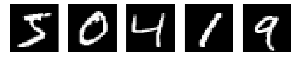
Let’s see what we get by normalizing images and compare them with the original outputs
X_ = normalize_input(X)

plots(X[:5]), plots(X_[:5])
(None, None)
The actual model
from keras.models import Sequential
from keras.layers.core import Lambda

from keras.layers import Dense, InputLayer, Flatten
from keras.optimizers import Adam

model = Sequential([
        Lambda(normalize_input, input_shape=(1, 28, 28)),
        Flatten(),
        Dense(10, activation='softmax')
    ])

model.compile(Adam(), loss='categorical_crossentropy', metrics=['accuracy'])
Let’s print the architecture to what we’ve defined
model.summary()
____________________________________________________________________________________________________
Layer (type)                     Output Shape          Param #     Connected to
====================================================================================================
lambda_2 (Lambda)                (None, 1, 28, 28)     0           lambda_input_2[0][0]
____________________________________________________________________________________________________
flatten_4 (Flatten)              (None, 784)           0           lambda_2[0][0]
____________________________________________________________________________________________________
dense_5 (Dense)                  (None, 10)            7850        flatten_4[0][0]
====================================================================================================
Total params: 7850
____________________________________________________________________________________________________
Train!!
model.fit(X, y, nb_epoch=5, validation_data=(X_val, y_val))
Train on 60000 samples, validate on 10000 samples
Epoch 1/5
60000/60000 [==============================] - 3s - loss: 0.3871 - acc: 0.8859 - val_loss: 0.2986 - val_acc: 0.9146
Epoch 2/5
60000/60000 [==============================] - 3s - loss: 0.3004 - acc: 0.9151 - val_loss: 0.2856 - val_acc: 0.9171
Epoch 3/5
60000/60000 [==============================] - 3s - loss: 0.2872 - acc: 0.9201 - val_loss: 0.3002 - val_acc: 0.9169
Epoch 4/5
60000/60000 [==============================] - 3s - loss: 0.2819 - acc: 0.9209 - val_loss: 0.2851 - val_acc: 0.9190
Epoch 5/5
60000/60000 [==============================] - 3s - loss: 0.2762 - acc: 0.9231 - val_loss: 0.2921 - val_acc: 0.9195


<keras.callbacks.History at 0x7f7fe26ed9d0>
Result
92.44%
Model 3: One hidden layer, going deep
Now the above is nice but it’s kind of bad. 92% accuracy is so ’90s.
One obvious way to improve it is to add another layer hidden layer. This adds a whole lot of new flexibility.
Model implementation
model = Sequential([
        Lambda(normalize_input, input_shape=(1, 28, 28)),
        Flatten(),
        Dense(100, activation='sigmoid'),
        Dense(10, activation='softmax')
    ])

model.compile(Adam(), loss='categorical_crossentropy', metrics=['accuracy'])
model.summary()
____________________________________________________________________________________________________
Layer (type)                     Output Shape          Param #     Connected to
====================================================================================================
lambda_3 (Lambda)                (None, 1, 28, 28)     0           lambda_input_3[0][0]
____________________________________________________________________________________________________
flatten_5 (Flatten)              (None, 784)           0           lambda_3[0][0]
____________________________________________________________________________________________________
dense_6 (Dense)                  (None, 100)           78500       flatten_5[0][0]
____________________________________________________________________________________________________
dense_7 (Dense)                  (None, 10)            1010        dense_6[0][0]
====================================================================================================
Total params: 79510
____________________________________________________________________________________________________
model.fit(X, y, nb_epoch=5, validation_data=(X_val, y_val))
Train on 60000 samples, validate on 10000 samples
Epoch 1/5
60000/60000 [==============================] - 4s - loss: 0.0583 - acc: 0.9836 - val_loss: 0.0933 - val_acc: 0.9713
Epoch 2/5
60000/60000 [==============================] - 4s - loss: 0.0490 - acc: 0.9864 - val_loss: 0.0876 - val_acc: 0.9735
Epoch 3/5
60000/60000 [==============================] - 4s - loss: 0.0416 - acc: 0.9885 - val_loss: 0.0833 - val_acc: 0.9759
Epoch 4/5
60000/60000 [==============================] - 4s - loss: 0.0353 - acc: 0.9908 - val_loss: 0.0864 - val_acc: 0.9746
Epoch 5/5
60000/60000 [==============================] - 4s - loss: 0.0301 - acc: 0.9920 - val_loss: 0.0846 - val_acc: 0.9748


<keras.callbacks.History at 0x7f7fe13e7ed0>
Result
97.03%
Notice that the amount of varibles start to increase..
Model 4: Even more layers
Let’s add even more layers, this time using relu as an activation function.
If we have even 3 layers, then we already have a model with hundreds of thousands of paramters…
Model implementation
model = Sequential([
        Lambda(normalize_input, input_shape=(1, 28, 28)),
        Flatten(),
        Dense(200, activation='relu'),
        Dense(200, activation='relu'),
        Dense(200, activation='relu'),
        Dense(10, activation='softmax')
    ])

model.compile(Adam(), loss='categorical_crossentropy', metrics=['accuracy'])
model.summary()
____________________________________________________________________________________________________
Layer (type)                     Output Shape          Param #     Connected to
====================================================================================================
lambda_4 (Lambda)                (None, 1, 28, 28)     0           lambda_input_4[0][0]
____________________________________________________________________________________________________
flatten_6 (Flatten)              (None, 784)           0           lambda_4[0][0]
____________________________________________________________________________________________________
dense_8 (Dense)                  (None, 200)           157000      flatten_6[0][0]
____________________________________________________________________________________________________
dense_9 (Dense)                  (None, 200)           40200       dense_8[0][0]
____________________________________________________________________________________________________
dense_10 (Dense)                 (None, 200)           40200       dense_9[0][0]
____________________________________________________________________________________________________
dense_11 (Dense)                 (None, 10)            2010        dense_10[0][0]
====================================================================================================
Total params: 239410
____________________________________________________________________________________________________
It’s almost certain that the model will overfitt badly.
model.fit(X, y, validation_data=(X_val, y_val), nb_epoch=5)
Train on 60000 samples, validate on 10000 samples
Epoch 1/5
60000/60000 [==============================] - 8s - loss: 0.2084 - acc: 0.9359 - val_loss: 0.1232 - val_acc: 0.9641
Epoch 2/5
60000/60000 [==============================] - 8s - loss: 0.1029 - acc: 0.9684 - val_loss: 0.1494 - val_acc: 0.9545
Epoch 3/5
60000/60000 [==============================] - 8s - loss: 0.0800 - acc: 0.9751 - val_loss: 0.1078 - val_acc: 0.9712
Epoch 4/5
60000/60000 [==============================] - 8s - loss: 0.0634 - acc: 0.9799 - val_loss: 0.0928 - val_acc: 0.9720
Epoch 5/5
60000/60000 [==============================] - 8s - loss: 0.0523 - acc: 0.9834 - val_loss: 0.1241 - val_acc: 0.9688


<keras.callbacks.History at 0x7f7fe059c5d0>
Result
97.75%
Model 5: Convolutions
To have a cleaner(smaller) model we need to use something more semantically meaningfull, such as a convolution.
What is a convolution?
- Consider it a sliding window over the image.
- The window is (maybe) 3x3 and it detects certain patterns, like a line, or a corner
- Sliding this window over the full image, yields a certain way of looking at the original image, like a filter.
- That’s actually what they are called.
- So a small window (3x3) creates a filtered image.
- We can have more filters, like expanding our initial image into multiple ways of looking at it
- Has anyone here seen the Predator series? … something like that
Model implementation
from keras.layers.convolutional import Convolution2D, MaxPooling2D

model = Sequential([
        Lambda(normalize_input, input_shape=(1, 28, 28)),
        Convolution2D(7, 3, 3, activation='relu', border_mode='same'),
        Convolution2D(7, 3, 3, activation='relu', border_mode='same'),
        Convolution2D(7, 3, 3, activation='relu', border_mode='same'),
        Flatten(),
        Dense(10, activation='softmax')
    ])

model.compile(Adam(), loss='categorical_crossentropy', metrics=['accuracy'])
model.summary()
____________________________________________________________________________________________________
Layer (type)                     Output Shape          Param #     Connected to
====================================================================================================
lambda_5 (Lambda)                (None, 1, 28, 28)     0           lambda_input_5[0][0]
____________________________________________________________________________________________________
convolution2d_11 (Convolution2D) (None, 7, 28, 28)     70          lambda_5[0][0]
____________________________________________________________________________________________________
convolution2d_12 (Convolution2D) (None, 7, 28, 28)     448         convolution2d_11[0][0]
____________________________________________________________________________________________________
convolution2d_13 (Convolution2D) (None, 7, 28, 28)     448         convolution2d_12[0][0]
____________________________________________________________________________________________________
flatten_7 (Flatten)              (None, 5488)          0           convolution2d_13[0][0]
____________________________________________________________________________________________________
dense_12 (Dense)                 (None, 10)            54890       flatten_7[0][0]
====================================================================================================
Total params: 55856
____________________________________________________________________________________________________
Only 55k parameters, that’s nice. But will it train?
model.fit(X, y, validation_data=(X_val, y_val), nb_epoch=5)
Train on 60000 samples, validate on 10000 samples
Epoch 1/5
60000/60000 [==============================] - 22s - loss: 0.1646 - acc: 0.9506 - val_loss: 0.0733 - val_acc: 0.9772
Epoch 2/5
60000/60000 [==============================] - 22s - loss: 0.0691 - acc: 0.9787 - val_loss: 0.0735 - val_acc: 0.9769
Epoch 3/5
60000/60000 [==============================] - 23s - loss: 0.0510 - acc: 0.9839 - val_loss: 0.0497 - val_acc: 0.9835
Epoch 4/5
60000/60000 [==============================] - 22s - loss: 0.0385 - acc: 0.9879 - val_loss: 0.0645 - val_acc: 0.9803
Epoch 5/5
60000/60000 [==============================] - 22s - loss: 0.0292 - acc: 0.9909 - val_loss: 0.0629 - val_acc: 0.9822


<keras.callbacks.History at 0x7f7fd759c610>
Result
98.49%
Model 6: MaxPooling
Using many convolutions, we still get a lot of paramters. Even more so if we consider that correctly representing an object requires has many different filters and compositions of them.
And now the problem with more convolutions is even not as much about the memmory, but the time of a single epoch.
A convolution is really slow, compared to a Dense layer!
A way to scale back on the problem is to decrease the input size of the convolutions so there is less space for the convolution window to travel.
This is what MaxPooling does.
What is MaxPooling
- Takes a matrix as input and outputs the maximum number of it.
- If the matrix is 2x2 than it makes the network 2 times smaller
a = np.array([[1, 2], [1, 3]])
a, np.max(a)
(array([[1, 2],
        [1, 3]]), 3)
Model implementation
from keras.layers.convolutional import Convolution2D, MaxPooling2D

model = Sequential([
        Lambda(normalize_input, input_shape=(1, 28, 28)),
        Convolution2D(7, 3, 3, activation='relu', border_mode='same'),
        MaxPooling2D(pool_size=(2,2), strides=(2,2), dim_ordering='th'),
        Convolution2D(14, 3, 3, activation='relu', border_mode='same'),
        MaxPooling2D(pool_size=(2,2), strides=(2,2), dim_ordering='th'),
        Convolution2D(28, 3, 3, activation='relu', border_mode='same'),
        MaxPooling2D(pool_size=(2,2), strides=(2,2), dim_ordering='th'),
        Convolution2D(28, 3, 3, activation='relu', border_mode='same'),
        Flatten(),
        Dense(10, activation='softmax')
    ])

model.compile(Adam(), loss='categorical_crossentropy', metrics=['accuracy'])
model.summary()
____________________________________________________________________________________________________
Layer (type)                     Output Shape          Param #     Connected to
====================================================================================================
lambda_6 (Lambda)                (None, 1, 28, 28)     0           lambda_input_6[0][0]
____________________________________________________________________________________________________
convolution2d_14 (Convolution2D) (None, 7, 28, 28)     70          lambda_6[0][0]
____________________________________________________________________________________________________
maxpooling2d_5 (MaxPooling2D)    (None, 7, 14, 14)     0           convolution2d_14[0][0]
____________________________________________________________________________________________________
convolution2d_15 (Convolution2D) (None, 14, 14, 14)    896         maxpooling2d_5[0][0]
____________________________________________________________________________________________________
maxpooling2d_6 (MaxPooling2D)    (None, 14, 7, 7)      0           convolution2d_15[0][0]
____________________________________________________________________________________________________
convolution2d_16 (Convolution2D) (None, 28, 7, 7)      3556        maxpooling2d_6[0][0]
____________________________________________________________________________________________________
maxpooling2d_7 (MaxPooling2D)    (None, 28, 3, 3)      0           convolution2d_16[0][0]
____________________________________________________________________________________________________
convolution2d_17 (Convolution2D) (None, 28, 3, 3)      7084        maxpooling2d_7[0][0]
____________________________________________________________________________________________________
flatten_8 (Flatten)              (None, 252)           0           convolution2d_17[0][0]
____________________________________________________________________________________________________
dense_13 (Dense)                 (None, 10)            2530        flatten_8[0][0]
====================================================================================================
Total params: 14136
____________________________________________________________________________________________________
model.fit(X, y, validation_data=(X_val, y_val), nb_epoch=5)
Train on 60000 samples, validate on 10000 samples
Epoch 1/5
60000/60000 [==============================] - 15s - loss: 0.1865 - acc: 0.9441 - val_loss: 0.0627 - val_acc: 0.9787
Epoch 2/5
60000/60000 [==============================] - 15s - loss: 0.0590 - acc: 0.9815 - val_loss: 0.0416 - val_acc: 0.9864
Epoch 3/5
60000/60000 [==============================] - 15s - loss: 0.0434 - acc: 0.9867 - val_loss: 0.0463 - val_acc: 0.9841
Epoch 4/5
60000/60000 [==============================] - 15s - loss: 0.0360 - acc: 0.9885 - val_loss: 0.0482 - val_acc: 0.9849
Epoch 5/5
60000/60000 [==============================] - 15s - loss: 0.0295 - acc: 0.9905 - val_loss: 0.0499 - val_acc: 0.9838


<keras.callbacks.History at 0x7f7fe1bd6790>
Result
98.37%
Model 7: Vgg style
Vgg is an architecture proposed by the Oxford team in 2014 on the ImageNet competition.
Even though it didn’t won that year’s competition, it was really close behind and more than that it had such a simple and clean architecture that made it really popular in the deep learning comunity.
The conceptual idea of Vgg is stacking blocks of convolutions, them MaxPooling once in a while. Then add a Dense layer to provide ways for the network to compose the resulting filters.
Model implementation
from keras.layers.convolutional import Convolution2D, MaxPooling2D

model = Sequential([
        Lambda(normalize_input, input_shape=(1, 28, 28)),
        Convolution2D(7, 3, 3, activation='relu', border_mode='same'),
        Convolution2D(7, 3, 3, activation='relu', border_mode='same'),
        MaxPooling2D(pool_size=(2,2), strides=(2,2), dim_ordering='th'),
        Convolution2D(14, 3, 3, activation='relu', border_mode='same'),
        Convolution2D(14, 3, 3, activation='relu', border_mode='same'),
        MaxPooling2D(pool_size=(2,2), strides=(2,2), dim_ordering='th'),
        Convolution2D(28, 3, 3, activation='relu', border_mode='same'),
        Convolution2D(28, 3, 3, activation='relu', border_mode='same'),
        Convolution2D(28, 3, 3, activation='relu', border_mode='same'),
        MaxPooling2D(pool_size=(2,2), strides=(2,2), dim_ordering='th'),
        Convolution2D(56, 3, 3, activation='relu', border_mode='same'),
        Convolution2D(56, 3, 3, activation='relu', border_mode='same'),
        Convolution2D(56, 3, 3, activation='relu', border_mode='same'),
        MaxPooling2D(pool_size=(2,2), strides=(2,2), dim_ordering='th'),
        Flatten(),
        Dense(100, activation='sigmoid'),
        Dense(10, activation='softmax')
    ])

model.compile(Adam(), loss='categorical_crossentropy', metrics=['accuracy'])
model.summary()
____________________________________________________________________________________________________
Layer (type)                     Output Shape          Param #     Connected to
====================================================================================================
lambda_7 (Lambda)                (None, 1, 28, 28)     0           lambda_input_7[0][0]
____________________________________________________________________________________________________
convolution2d_18 (Convolution2D) (None, 7, 28, 28)     70          lambda_7[0][0]
____________________________________________________________________________________________________
convolution2d_19 (Convolution2D) (None, 7, 28, 28)     448         convolution2d_18[0][0]
____________________________________________________________________________________________________
maxpooling2d_8 (MaxPooling2D)    (None, 7, 14, 14)     0           convolution2d_19[0][0]
____________________________________________________________________________________________________
convolution2d_20 (Convolution2D) (None, 14, 14, 14)    896         maxpooling2d_8[0][0]
____________________________________________________________________________________________________
convolution2d_21 (Convolution2D) (None, 14, 14, 14)    1778        convolution2d_20[0][0]
____________________________________________________________________________________________________
maxpooling2d_9 (MaxPooling2D)    (None, 14, 7, 7)      0           convolution2d_21[0][0]
____________________________________________________________________________________________________
convolution2d_22 (Convolution2D) (None, 28, 7, 7)      3556        maxpooling2d_9[0][0]
____________________________________________________________________________________________________
convolution2d_23 (Convolution2D) (None, 28, 7, 7)      7084        convolution2d_22[0][0]
____________________________________________________________________________________________________
convolution2d_24 (Convolution2D) (None, 28, 7, 7)      7084        convolution2d_23[0][0]
____________________________________________________________________________________________________
maxpooling2d_10 (MaxPooling2D)   (None, 28, 3, 3)      0           convolution2d_24[0][0]
____________________________________________________________________________________________________
convolution2d_25 (Convolution2D) (None, 56, 3, 3)      14168       maxpooling2d_10[0][0]
____________________________________________________________________________________________________
convolution2d_26 (Convolution2D) (None, 56, 3, 3)      28280       convolution2d_25[0][0]
____________________________________________________________________________________________________
convolution2d_27 (Convolution2D) (None, 56, 3, 3)      28280       convolution2d_26[0][0]
____________________________________________________________________________________________________
maxpooling2d_11 (MaxPooling2D)   (None, 56, 1, 1)      0           convolution2d_27[0][0]
____________________________________________________________________________________________________
flatten_9 (Flatten)              (None, 56)            0           maxpooling2d_11[0][0]
____________________________________________________________________________________________________
dense_14 (Dense)                 (None, 100)           5700        flatten_9[0][0]
____________________________________________________________________________________________________
dense_15 (Dense)                 (None, 10)            1010        dense_14[0][0]
====================================================================================================
Total params: 98354
____________________________________________________________________________________________________
model.fit(X, y, validation_data=(X_val, y_val), nb_epoch=4)
Train on 60000 samples, validate on 10000 samples
Epoch 1/4
60000/60000 [==============================] - 40s - loss: 0.2940 - acc: 0.9083 - val_loss: 0.0816 - val_acc: 0.9764
Epoch 2/4
60000/60000 [==============================] - 40s - loss: 0.0747 - acc: 0.9787 - val_loss: 0.0552 - val_acc: 0.9835
Epoch 3/4
60000/60000 [==============================] - 40s - loss: 0.0555 - acc: 0.9839 - val_loss: 0.0587 - val_acc: 0.9826
Epoch 4/4
60000/60000 [==============================] - 40s - loss: 0.0509 - acc: 0.9856 - val_loss: 0.0731 - val_acc: 0.9782


<keras.callbacks.History at 0x7f7fcdefbc10>
Result
96.94%
Model 8: BatchNormalization
- Usually, we do normalization of the input data by: data = data - mean(data) / stddev(data)
- We can’t do this on each layer output because they’re not static data
- Adaptively learn the std and mean on each layer as a pair of tunnable parameters
Model implementation
from keras.layers.convolutional import Convolution2D, MaxPooling2D
from keras.layers.normalization import BatchNormalization

model = Sequential([
        Lambda(normalize_input, input_shape=(1, 28, 28)),
        Convolution2D(7, 3, 3, activation='relu', border_mode='same'),
        Convolution2D(7, 3, 3, activation='relu', border_mode='same'),
        MaxPooling2D(pool_size=(2,2), strides=(2,2), dim_ordering='th'),
        BatchNormalization(axis=1),
        Convolution2D(14, 3, 3, activation='relu', border_mode='same'),
        Convolution2D(14, 3, 3, activation='relu', border_mode='same'),
        MaxPooling2D(pool_size=(2,2), strides=(2,2), dim_ordering='th'),
        BatchNormalization(axis=1),
        Convolution2D(28, 3, 3, activation='relu', border_mode='same'),
        Convolution2D(28, 3, 3, activation='relu', border_mode='same'),
        Convolution2D(28, 3, 3, activation='relu', border_mode='same'),
        MaxPooling2D(pool_size=(2,2), strides=(2,2), dim_ordering='th'),
        BatchNormalization(axis=1),
        Convolution2D(56, 3, 3, activation='relu', border_mode='same'),
        Convolution2D(56, 3, 3, activation='relu', border_mode='same'),
        Convolution2D(56, 3, 3, activation='relu', border_mode='same'),
        MaxPooling2D(pool_size=(2,2), strides=(2,2), dim_ordering='th'),
        BatchNormalization(axis=1),
        Flatten(),
        Dense(100, activation='sigmoid'),
        Dense(10, activation='softmax')
    ])

model.compile(Adam(), loss='categorical_crossentropy', metrics=['accuracy'])
model.summary()
____________________________________________________________________________________________________
Layer (type)                     Output Shape          Param #     Connected to
====================================================================================================
lambda_19 (Lambda)               (None, 1, 28, 28)     0           lambda_input_19[0][0]
____________________________________________________________________________________________________
convolution2d_39 (Convolution2D) (None, 7, 28, 28)     70          lambda_19[0][0]
____________________________________________________________________________________________________
convolution2d_40 (Convolution2D) (None, 7, 28, 28)     448         convolution2d_39[0][0]
____________________________________________________________________________________________________
maxpooling2d_16 (MaxPooling2D)   (None, 7, 14, 14)     0           convolution2d_40[0][0]
____________________________________________________________________________________________________
batchnormalization_1 (BatchNormal(None, 7, 14, 14)     14          maxpooling2d_16[0][0]
____________________________________________________________________________________________________
convolution2d_41 (Convolution2D) (None, 14, 14, 14)    896         batchnormalization_1[0][0]
____________________________________________________________________________________________________
convolution2d_42 (Convolution2D) (None, 14, 14, 14)    1778        convolution2d_41[0][0]
____________________________________________________________________________________________________
maxpooling2d_17 (MaxPooling2D)   (None, 14, 7, 7)      0           convolution2d_42[0][0]
____________________________________________________________________________________________________
batchnormalization_2 (BatchNormal(None, 14, 7, 7)      28          maxpooling2d_17[0][0]
____________________________________________________________________________________________________
convolution2d_43 (Convolution2D) (None, 28, 7, 7)      3556        batchnormalization_2[0][0]
____________________________________________________________________________________________________
convolution2d_44 (Convolution2D) (None, 28, 7, 7)      7084        convolution2d_43[0][0]
____________________________________________________________________________________________________
convolution2d_45 (Convolution2D) (None, 28, 7, 7)      7084        convolution2d_44[0][0]
____________________________________________________________________________________________________
maxpooling2d_18 (MaxPooling2D)   (None, 28, 3, 3)      0           convolution2d_45[0][0]
____________________________________________________________________________________________________
batchnormalization_3 (BatchNormal(None, 28, 3, 3)      56          maxpooling2d_18[0][0]
____________________________________________________________________________________________________
convolution2d_46 (Convolution2D) (None, 56, 3, 3)      14168       batchnormalization_3[0][0]
____________________________________________________________________________________________________
convolution2d_47 (Convolution2D) (None, 56, 3, 3)      28280       convolution2d_46[0][0]
____________________________________________________________________________________________________
convolution2d_48 (Convolution2D) (None, 56, 3, 3)      28280       convolution2d_47[0][0]
____________________________________________________________________________________________________
maxpooling2d_19 (MaxPooling2D)   (None, 56, 1, 1)      0           convolution2d_48[0][0]
____________________________________________________________________________________________________
batchnormalization_4 (BatchNormal(None, 56, 1, 1)      112         maxpooling2d_19[0][0]
____________________________________________________________________________________________________
flatten_21 (Flatten)             (None, 56)            0           batchnormalization_4[0][0]
____________________________________________________________________________________________________
dense_34 (Dense)                 (None, 100)           5700        flatten_21[0][0]
____________________________________________________________________________________________________
dense_35 (Dense)                 (None, 10)            1010        dense_34[0][0]
====================================================================================================
Total params: 98564
____________________________________________________________________________________________________
model.fit(X, y, validation_data=(X_val, y_val), nb_epoch=5)
Train on 60000 samples, validate on 10000 samples
Epoch 1/5
60000/60000 [==============================] - 52s - loss: 0.1731 - acc: 0.9561 - val_loss: 0.0850 - val_acc: 0.9751
Epoch 2/5
60000/60000 [==============================] - 52s - loss: 0.0594 - acc: 0.9826 - val_loss: 0.0763 - val_acc: 0.9782
Epoch 3/5
60000/60000 [==============================] - 52s - loss: 0.0461 - acc: 0.9862 - val_loss: 0.0604 - val_acc: 0.9816
Epoch 4/5
60000/60000 [==============================] - 52s - loss: 0.0379 - acc: 0.9888 - val_loss: 0.0387 - val_acc: 0.9893
Epoch 5/5
60000/60000 [==============================] - 52s - loss: 0.0323 - acc: 0.9900 - val_loss: 0.0970 - val_acc: 0.9712


<keras.callbacks.History at 0x7f9aa91cc710>
Result
98.93%
Model 9: Regularisation. Dropout
We’ve seen that by now, the network starts to overfit.
Adding means by which the network is able to learn meaningfull stuff is called regularization.
One way of doing it is to use Dropout.
What is Dropout?
A layer that randomly makes a percentage of the inputs 0 and outputs the result.
def dropout(a, percentage):
    b = np.copy(a)
    choose = np.random.permutation(np.arange(len(a)))[:int(len(a) * percentage)]

    # make some 0
    b[choose] = 0
    return b

dropout(np.arange(10), 0.4)
array([0, 0, 2, 0, 4, 5, 6, 0, 8, 0])
By doing this no node will be able to specialize in for exactly one example. Instead it will learn something usefull from a sample of the training set.
Model implementation
from keras.layers.convolutional import Convolution2D, MaxPooling2D
from keras.layers.normalization import BatchNormalization
from keras.layers.core import Dropout

model = Sequential([
        Lambda(normalize_input, input_shape=(1, 28, 28)),
        Convolution2D(7, 3, 3, activation='relu', border_mode='same'),
        Convolution2D(7, 3, 3, activation='relu', border_mode='same'),
        MaxPooling2D(pool_size=(2,2), strides=(2,2), dim_ordering='th'),
        BatchNormalization(axis=1),
        Dropout(0.1),
        Convolution2D(14, 3, 3, activation='relu', border_mode='same'),
        Convolution2D(14, 3, 3, activation='relu', border_mode='same'),
        MaxPooling2D(pool_size=(2,2), strides=(2,2), dim_ordering='th'),
        BatchNormalization(axis=1),
        Dropout(0.2),
        Convolution2D(28, 3, 3, activation='relu', border_mode='same'),
        Convolution2D(28, 3, 3, activation='relu', border_mode='same'),
        Convolution2D(28, 3, 3, activation='relu', border_mode='same'),
        MaxPooling2D(pool_size=(2,2), strides=(2,2), dim_ordering='th'),
        BatchNormalization(axis=1),
        Dropout(0.3),
        Convolution2D(56, 3, 3, activation='relu', border_mode='same'),
        Convolution2D(56, 3, 3, activation='relu', border_mode='same'),
        Convolution2D(56, 3, 3, activation='relu', border_mode='same'),
        MaxPooling2D(pool_size=(2,2), strides=(2,2), dim_ordering='th'),
        BatchNormalization(axis=1),
        Dropout(0.4),
        Flatten(),
        Dense(100, activation='sigmoid'),
        Dropout(0.5),
        Dense(10, activation='softmax')
    ])

model.compile(Adam(), loss='categorical_crossentropy', metrics=['accuracy'])
model.summary()
____________________________________________________________________________________________________
Layer (type)                     Output Shape          Param #     Connected to
====================================================================================================
lambda_21 (Lambda)               (None, 1, 28, 28)     0           lambda_input_20[0][0]
____________________________________________________________________________________________________
convolution2d_51 (Convolution2D) (None, 7, 28, 28)     70          lambda_21[0][0]
____________________________________________________________________________________________________
convolution2d_52 (Convolution2D) (None, 7, 28, 28)     448         convolution2d_51[0][0]
____________________________________________________________________________________________________
maxpooling2d_21 (MaxPooling2D)   (None, 7, 14, 14)     0           convolution2d_52[0][0]
____________________________________________________________________________________________________
batchnormalization_6 (BatchNormal(None, 7, 14, 14)     14          maxpooling2d_21[0][0]
____________________________________________________________________________________________________
dropout_1 (Dropout)              (None, 7, 14, 14)     0           batchnormalization_6[0][0]
____________________________________________________________________________________________________
convolution2d_53 (Convolution2D) (None, 14, 14, 14)    896         dropout_1[0][0]
____________________________________________________________________________________________________
convolution2d_54 (Convolution2D) (None, 14, 14, 14)    1778        convolution2d_53[0][0]
____________________________________________________________________________________________________
maxpooling2d_22 (MaxPooling2D)   (None, 14, 7, 7)      0           convolution2d_54[0][0]
____________________________________________________________________________________________________
batchnormalization_7 (BatchNormal(None, 14, 7, 7)      28          maxpooling2d_22[0][0]
____________________________________________________________________________________________________
dropout_2 (Dropout)              (None, 14, 7, 7)      0           batchnormalization_7[0][0]
____________________________________________________________________________________________________
convolution2d_55 (Convolution2D) (None, 28, 7, 7)      3556        dropout_2[0][0]
____________________________________________________________________________________________________
convolution2d_56 (Convolution2D) (None, 28, 7, 7)      7084        convolution2d_55[0][0]
____________________________________________________________________________________________________
convolution2d_57 (Convolution2D) (None, 28, 7, 7)      7084        convolution2d_56[0][0]
____________________________________________________________________________________________________
maxpooling2d_23 (MaxPooling2D)   (None, 28, 3, 3)      0           convolution2d_57[0][0]
____________________________________________________________________________________________________
batchnormalization_8 (BatchNormal(None, 28, 3, 3)      56          maxpooling2d_23[0][0]
____________________________________________________________________________________________________
dropout_3 (Dropout)              (None, 28, 3, 3)      0           batchnormalization_8[0][0]
____________________________________________________________________________________________________
convolution2d_58 (Convolution2D) (None, 56, 3, 3)      14168       dropout_3[0][0]
____________________________________________________________________________________________________
convolution2d_59 (Convolution2D) (None, 56, 3, 3)      28280       convolution2d_58[0][0]
____________________________________________________________________________________________________
convolution2d_60 (Convolution2D) (None, 56, 3, 3)      28280       convolution2d_59[0][0]
____________________________________________________________________________________________________
maxpooling2d_24 (MaxPooling2D)   (None, 56, 1, 1)      0           convolution2d_60[0][0]
____________________________________________________________________________________________________
batchnormalization_9 (BatchNormal(None, 56, 1, 1)      112         maxpooling2d_24[0][0]
____________________________________________________________________________________________________
dropout_4 (Dropout)              (None, 56, 1, 1)      0           batchnormalization_9[0][0]
____________________________________________________________________________________________________
flatten_22 (Flatten)             (None, 56)            0           dropout_4[0][0]
____________________________________________________________________________________________________
dense_36 (Dense)                 (None, 100)           5700        flatten_22[0][0]
____________________________________________________________________________________________________
dropout_5 (Dropout)              (None, 100)           0           dense_36[0][0]
____________________________________________________________________________________________________
dense_37 (Dense)                 (None, 10)            1010        dropout_5[0][0]
====================================================================================================
Total params: 98564
____________________________________________________________________________________________________
model.fit(X, y, validation_data=(X_val, y_val), nb_epoch=5)
Train on 60000 samples, validate on 10000 samples
Epoch 1/5
60000/60000 [==============================] - 57s - loss: 0.4139 - acc: 0.8825 - val_loss: 0.0677 - val_acc: 0.9804
Epoch 2/5
60000/60000 [==============================] - 57s - loss: 0.1287 - acc: 0.9691 - val_loss: 0.0559 - val_acc: 0.9839
Epoch 3/5
60000/60000 [==============================] - 57s - loss: 0.0990 - acc: 0.9760 - val_loss: 0.0450 - val_acc: 0.9885
Epoch 4/5
60000/60000 [==============================] - 57s - loss: 0.0809 - acc: 0.9804 - val_loss: 0.0428 - val_acc: 0.9896
Epoch 5/5
60000/60000 [==============================] - 57s - loss: 0.0723 - acc: 0.9816 - val_loss: 0.0378 - val_acc: 0.9898


<keras.callbacks.History at 0x7f9a9afd2110>
Result
98.98%
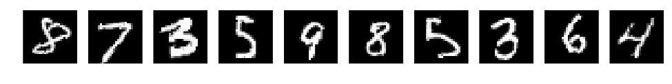
Model 10: Data augmentation
Using only the data that we are provided is fair.
But our goal is to have a good, usable model that generalizes well so we can augment the trainin data.
We can use the following trainsformation for example:
- shrinkage
- skewing
- retation
- translation
- color shifting, etc..
This basically generates infinite amount of labeled training data and makes the model much better.
Data augmentation in keras
from keras.preprocessing.image import ImageDataGenerator
gen = ImageDataGenerator(rotation_range=10, zoom_range=0.1, shear_range=0.1, dim_ordering='th')
batch_gen = gen.flow(X, y, batch_size=128)
img, _ = next(batch_gen)
plots(img[:10])
print(batch_gen.N)
60000
Model implementation
from keras.layers.convolutional import Convolution2D, MaxPooling2D
from keras.layers.normalization import BatchNormalization
from keras.layers.core import Dropout

model = Sequential([
        Lambda(normalize_input, input_shape=(1, 28, 28)),
        Convolution2D(7, 3, 3, activation='relu', border_mode='same'),
        Convolution2D(7, 3, 3, activation='relu', border_mode='same'),
        MaxPooling2D(pool_size=(2,2), strides=(2,2), dim_ordering='th'),
        BatchNormalization(axis=1),
        Dropout(0.1),
        Convolution2D(14, 3, 3, activation='relu', border_mode='same'),
        Convolution2D(14, 3, 3, activation='relu', border_mode='same'),
        MaxPooling2D(pool_size=(2,2), strides=(2,2), dim_ordering='th'),
        BatchNormalization(axis=1),
        Dropout(0.2),
        Convolution2D(28, 3, 3, activation='relu', border_mode='same'),
        Convolution2D(28, 3, 3, activation='relu', border_mode='same'),
        Convolution2D(28, 3, 3, activation='relu', border_mode='same'),
        MaxPooling2D(pool_size=(2,2), strides=(2,2), dim_ordering='th'),
        BatchNormalization(axis=1),
        Dropout(0.3),
        Convolution2D(56, 3, 3, activation='relu', border_mode='same'),
        Convolution2D(56, 3, 3, activation='relu', border_mode='same'),
        Convolution2D(56, 3, 3, activation='relu', border_mode='same'),
        MaxPooling2D(pool_size=(2,2), strides=(2,2), dim_ordering='th'),
        BatchNormalization(axis=1),
        Dropout(0.4),
        Flatten(),
        Dense(100, activation='sigmoid'),
        Dropout(0.5),
        Dense(10, activation='softmax')
    ])

model.compile(Adam(), loss='categorical_crossentropy', metrics=['accuracy'])
model.summary()
model.fit_generator(batch_gen, batch_gen.N, nb_epoch=10, validation_data=(X_val, y_val))
Epoch 1/10
60000/60000 [==============================] - 34s - loss: 0.7929 - acc: 0.7602 - val_loss: 0.1125 - val_acc: 0.9683
Epoch 2/10
60000/60000 [==============================] - 35s - loss: 0.1968 - acc: 0.9515 - val_loss: 0.0566 - val_acc: 0.9846
Epoch 3/10
60000/60000 [==============================] - 34s - loss: 0.1416 - acc: 0.9649 - val_loss: 0.0475 - val_acc: 0.9879
Epoch 4/10
60000/60000 [==============================] - 34s - loss: 0.1133 - acc: 0.9716 - val_loss: 0.0423 - val_acc: 0.9876
Epoch 5/10
60000/60000 [==============================] - 35s - loss: 0.1023 - acc: 0.9742 - val_loss: 0.0357 - val_acc: 0.9900
Epoch 6/10
60000/60000 [==============================] - 34s - loss: 0.0931 - acc: 0.9763 - val_loss: 0.0376 - val_acc: 0.9908
Epoch 7/10
60000/60000 [==============================] - 34s - loss: 0.0836 - acc: 0.9788 - val_loss: 0.0390 - val_acc: 0.9903
Epoch 8/10
60000/60000 [==============================] - 35s - loss: 0.0770 - acc: 0.9796 - val_loss: 0.0288 - val_acc: 0.9924
Epoch 9/10
60000/60000 [==============================] - 35s - loss: 0.0734 - acc: 0.9814 - val_loss: 0.0304 - val_acc: 0.9920
Epoch 10/10
60000/60000 [==============================] - 34s - loss: 0.0696 - acc: 0.9813 - val_loss: 0.0279 - val_acc: 0.9927


<keras.callbacks.History at 0x7f9a945c5b50>
Result
99.27%
Model 11: Training annealing
Train for some epochs and gradually reduce the learning rate because the network is already pretty well trained. You only need to slightly tune the outlier examples.
Model implementation
from keras.layers.convolutional import Convolution2D, MaxPooling2D
from keras.layers.normalization import BatchNormalization
from keras.layers.core import Dropout

model = Sequential([
        Lambda(normalize_input, input_shape=(1, 28, 28)),
        Convolution2D(7, 3, 3, activation='relu', border_mode='same'),
        Convolution2D(7, 3, 3, activation='relu', border_mode='same'),
        MaxPooling2D(pool_size=(2,2), strides=(2,2), dim_ordering='th'),
        BatchNormalization(axis=1),
        Dropout(0.1),
        Convolution2D(14, 3, 3, activation='relu', border_mode='same'),
        Convolution2D(14, 3, 3, activation='relu', border_mode='same'),
        MaxPooling2D(pool_size=(2,2), strides=(2,2), dim_ordering='th'),
        BatchNormalization(axis=1),
        Dropout(0.2),
        Convolution2D(28, 3, 3, activation='relu', border_mode='same'),
        Convolution2D(28, 3, 3, activation='relu', border_mode='same'),
        Convolution2D(28, 3, 3, activation='relu', border_mode='same'),
        MaxPooling2D(pool_size=(2,2), strides=(2,2), dim_ordering='th'),
        BatchNormalization(axis=1),
        Dropout(0.3),
        Convolution2D(56, 3, 3, activation='relu', border_mode='same'),
        Convolution2D(56, 3, 3, activation='relu', border_mode='same'),
        Convolution2D(56, 3, 3, activation='relu', border_mode='same'),
        MaxPooling2D(pool_size=(2,2), strides=(2,2), dim_ordering='th'),
        BatchNormalization(axis=1),
        Dropout(0.4),
        Flatten(),
        Dense(100, activation='sigmoid'),
        Dropout(0.5),
        Dense(10, activation='softmax')
    ])
model.compile(Adam(), loss='categorical_crossentropy', metrics=['accuracy'])
model.summary()
____________________________________________________________________________________________________
Layer (type)                     Output Shape          Param #     Connected to
====================================================================================================
lambda_1 (Lambda)                (None, 1, 28, 28)     0           lambda_input_1[0][0]
____________________________________________________________________________________________________
convolution2d_1 (Convolution2D)  (None, 7, 28, 28)     70          lambda_1[0][0]
____________________________________________________________________________________________________
convolution2d_2 (Convolution2D)  (None, 7, 28, 28)     448         convolution2d_1[0][0]
____________________________________________________________________________________________________
maxpooling2d_1 (MaxPooling2D)    (None, 7, 14, 14)     0           convolution2d_2[0][0]
____________________________________________________________________________________________________
batchnormalization_1 (BatchNormal(None, 7, 14, 14)     14          maxpooling2d_1[0][0]
____________________________________________________________________________________________________
dropout_1 (Dropout)              (None, 7, 14, 14)     0           batchnormalization_1[0][0]
____________________________________________________________________________________________________
convolution2d_3 (Convolution2D)  (None, 14, 14, 14)    896         dropout_1[0][0]
____________________________________________________________________________________________________
convolution2d_4 (Convolution2D)  (None, 14, 14, 14)    1778        convolution2d_3[0][0]
____________________________________________________________________________________________________
maxpooling2d_2 (MaxPooling2D)    (None, 14, 7, 7)      0           convolution2d_4[0][0]
____________________________________________________________________________________________________
batchnormalization_2 (BatchNormal(None, 14, 7, 7)      28          maxpooling2d_2[0][0]
____________________________________________________________________________________________________
dropout_2 (Dropout)              (None, 14, 7, 7)      0           batchnormalization_2[0][0]
____________________________________________________________________________________________________
convolution2d_5 (Convolution2D)  (None, 28, 7, 7)      3556        dropout_2[0][0]
____________________________________________________________________________________________________
convolution2d_6 (Convolution2D)  (None, 28, 7, 7)      7084        convolution2d_5[0][0]
____________________________________________________________________________________________________
convolution2d_7 (Convolution2D)  (None, 28, 7, 7)      7084        convolution2d_6[0][0]
____________________________________________________________________________________________________
maxpooling2d_3 (MaxPooling2D)    (None, 28, 3, 3)      0           convolution2d_7[0][0]
____________________________________________________________________________________________________
batchnormalization_3 (BatchNormal(None, 28, 3, 3)      56          maxpooling2d_3[0][0]
____________________________________________________________________________________________________
dropout_3 (Dropout)              (None, 28, 3, 3)      0           batchnormalization_3[0][0]
____________________________________________________________________________________________________
convolution2d_8 (Convolution2D)  (None, 56, 3, 3)      14168       dropout_3[0][0]
____________________________________________________________________________________________________
convolution2d_9 (Convolution2D)  (None, 56, 3, 3)      28280       convolution2d_8[0][0]
____________________________________________________________________________________________________
convolution2d_10 (Convolution2D) (None, 56, 3, 3)      28280       convolution2d_9[0][0]
____________________________________________________________________________________________________
maxpooling2d_4 (MaxPooling2D)    (None, 56, 1, 1)      0           convolution2d_10[0][0]
____________________________________________________________________________________________________
batchnormalization_4 (BatchNormal(None, 56, 1, 1)      112         maxpooling2d_4[0][0]
____________________________________________________________________________________________________
dropout_4 (Dropout)              (None, 56, 1, 1)      0           batchnormalization_4[0][0]
____________________________________________________________________________________________________
flatten_2 (Flatten)              (None, 56)            0           dropout_4[0][0]
____________________________________________________________________________________________________
dense_2 (Dense)                  (None, 100)           5700        flatten_2[0][0]
____________________________________________________________________________________________________
dropout_5 (Dropout)              (None, 100)           0           dense_2[0][0]
____________________________________________________________________________________________________
dense_3 (Dense)                  (None, 10)            1010        dropout_5[0][0]
====================================================================================================
Total params: 98564
____________________________________________________________________________________________________
model.optimizer.lr = 0.0001
model.fit(X, y, batch_size=64, nb_epoch=1, validation_data=(X_val, y_val))

model.optimizer.lr = 0.01
model.fit(X, y, batch_size=64, nb_epoch=3, validation_data=(X_val, y_val))

model.optimizer.lr = 0.01
model.fit_generator(batch_gen, batch_gen.N, nb_epoch=4, validation_data=(X_val, y_val))

model.optimizer.lr = 0.001
model.fit_generator(batch_gen, batch_gen.N, nb_epoch=5, validation_data=(X_val, y_val))

model.optimizer.lr = 0.0001
model.fit_generator(batch_gen, batch_gen.N, nb_epoch=5, validation_data=(X_val, y_val))

model.optimizer.lr = 0.00001
model.fit_generator(batch_gen, batch_gen.N, nb_epoch=5, validation_data=(X_val, y_val))
Train on 60000 samples, validate on 10000 samples
Epoch 1/1
60000/60000 [==============================] - 35s - loss: 1.7793 - acc: 0.4132 - val_loss: 0.6470 - val_acc: 0.8850
Train on 60000 samples, validate on 10000 samples
Epoch 1/3
60000/60000 [==============================] - 35s - loss: 0.7553 - acc: 0.8099 - val_loss: 0.2237 - val_acc: 0.9570
Epoch 2/3
60000/60000 [==============================] - 35s - loss: 0.3961 - acc: 0.9164 - val_loss: 0.1164 - val_acc: 0.9714
Epoch 3/3
60000/60000 [==============================] - 35s - loss: 0.2578 - acc: 0.9458 - val_loss: 0.0798 - val_acc: 0.9787
Epoch 1/4
60000/60000 [==============================] - 33s - loss: 0.2415 - acc: 0.9432 - val_loss: 0.0675 - val_acc: 0.9816
Epoch 2/4
60000/60000 [==============================] - 33s - loss: 0.2106 - acc: 0.9497 - val_loss: 0.0582 - val_acc: 0.9833
Epoch 3/4
60000/60000 [==============================] - 34s - loss: 0.1898 - acc: 0.9545 - val_loss: 0.0514 - val_acc: 0.9857
Epoch 4/4
60000/60000 [==============================] - 33s - loss: 0.1713 - acc: 0.9589 - val_loss: 0.0477 - val_acc: 0.9872
Epoch 1/5
60000/60000 [==============================] - 34s - loss: 0.1578 - acc: 0.9617 - val_loss: 0.0449 - val_acc: 0.9879
Epoch 2/5
60000/60000 [==============================] - 34s - loss: 0.1497 - acc: 0.9630 - val_loss: 0.0456 - val_acc: 0.9868
Epoch 3/5
60000/60000 [==============================] - 34s - loss: 0.1355 - acc: 0.9671 - val_loss: 0.0410 - val_acc: 0.9891
Epoch 4/5
60000/60000 [==============================] - 33s - loss: 0.1339 - acc: 0.9672 - val_loss: 0.0418 - val_acc: 0.9883
Epoch 5/5
60000/60000 [==============================] - 33s - loss: 0.1239 - acc: 0.9692 - val_loss: 0.0394 - val_acc: 0.9895
Epoch 1/5
60000/60000 [==============================] - 34s - loss: 0.1181 - acc: 0.9702 - val_loss: 0.0343 - val_acc: 0.9906
Epoch 2/5
60000/60000 [==============================] - 33s - loss: 0.1112 - acc: 0.9728 - val_loss: 0.0380 - val_acc: 0.9893
Epoch 3/5
60000/60000 [==============================] - 34s - loss: 0.1094 - acc: 0.9731 - val_loss: 0.0355 - val_acc: 0.9902
Epoch 4/5
60000/60000 [==============================] - 33s - loss: 0.1093 - acc: 0.9730 - val_loss: 0.0334 - val_acc: 0.9908
Epoch 5/5
60000/60000 [==============================] - 34s - loss: 0.0992 - acc: 0.9753 - val_loss: 0.0361 - val_acc: 0.9903
Epoch 1/5
60000/60000 [==============================] - 34s - loss: 0.0976 - acc: 0.9756 - val_loss: 0.0374 - val_acc: 0.9906
Epoch 2/5
60000/60000 [==============================] - 33s - loss: 0.0966 - acc: 0.9763 - val_loss: 0.0348 - val_acc: 0.9909
Epoch 3/5
60000/60000 [==============================] - 33s - loss: 0.0937 - acc: 0.9765 - val_loss: 0.0354 - val_acc: 0.9905
Epoch 4/5
60000/60000 [==============================] - 32s - loss: 0.0930 - acc: 0.9770 - val_loss: 0.0333 - val_acc: 0.9913
Epoch 5/5
60000/60000 [==============================] - 34s - loss: 0.0935 - acc: 0.9770 - val_loss: 0.0289 - val_acc: 0.9912


<keras.callbacks.History at 0x7f7ffbb0edd0>
model.optimizer.lr = 0.0000001
model.fit_generator(batch_gen, batch_gen.N, nb_epoch=5, validation_data=(X_val, y_val))
Epoch 1/5
60000/60000 [==============================] - 34s - loss: 0.0685 - acc: 0.9826 - val_loss: 0.0274 - val_acc: 0.9927
Epoch 2/5
60000/60000 [==============================] - 33s - loss: 0.0711 - acc: 0.9811 - val_loss: 0.0244 - val_acc: 0.9927
Epoch 3/5
60000/60000 [==============================] - 34s - loss: 0.0663 - acc: 0.9829 - val_loss: 0.0204 - val_acc: 0.9939
Epoch 4/5
60000/60000 [==============================] - 34s - loss: 0.0674 - acc: 0.9825 - val_loss: 0.0206 - val_acc: 0.9939
Epoch 5/5
60000/60000 [==============================] - 35s - loss: 0.0692 - acc: 0.9817 - val_loss: 0.0230 - val_acc: 0.9937


<keras.callbacks.History at 0x7f9a89fa80d0>
best_model = model
Result
99.39%
Model 12: Model averaging
The basic idea is to train multiple models, then use the predictions on all of them, average them toggeter and use that as the output.
This leads to approx. 15% improvements.
Result
99.5%
Model 13: Pseudo-labeling
- train a model with a resonable good accuracy
- use this model then to make predictions on all of our unlabelled data
- use those predictions as labels themselves
- be mindful of the proportion of true labels and psuedo-labels in each batch. Should be 1/4-1/3 of your batches be psuedo-labeled.
Should also add 10-15% to the accuracy.
Result
99.58%
Using the predictions
predictions = best_model.predict(X_val, X_val.shape[0])
labels_pred = np.argmax(predictions, axis=1)
labels = y_test
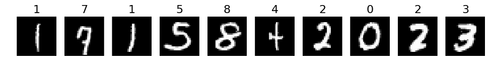
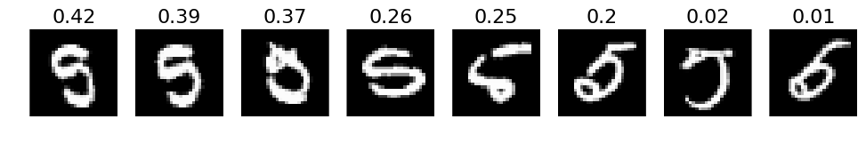
# 1. A few correct labels at random
print("Correct predictions")
correct = np.where(labels_pred == labels)[0]
correct = np.random.permutation(correct)
selected = correct[:10]
plots(X_val[selected], titles=labels_pred[selected])
Correct predictions
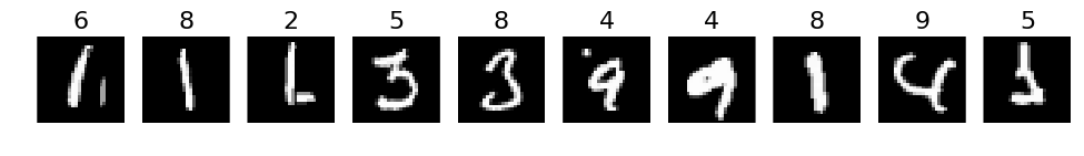
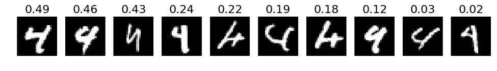
# 2. A few incorrect labels at random
print("Incorrect predictions")
incorrect = np.where(labels_pred != labels)[0]
incorrect = np.random.permutation(incorrect)
selected = incorrect[:10]
plots(X_val[selected], titles=labels_pred[selected])
Incorrect predictions
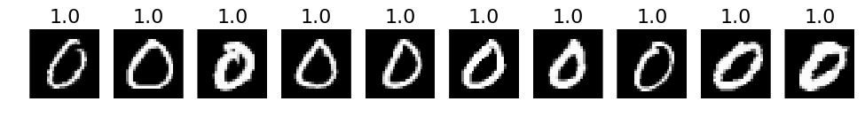
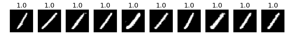
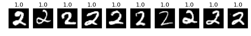
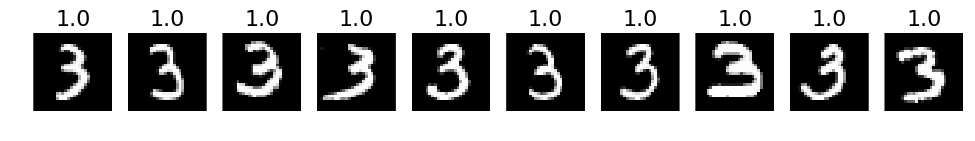
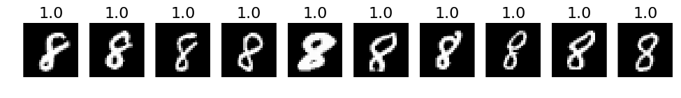
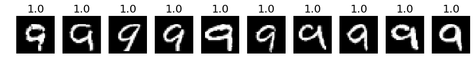
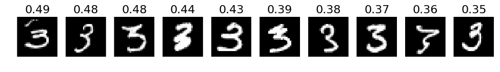
# 3. The most correct labeles (i.e. those with the highest probabilities that are correct)
def correct_labels(target_label, nr_sample):
    correct = np.where(labels_pred == labels)
    X_correct = X_val[correct]
    y_correct = y_test[correct]
    pred_correct = predictions[correct]

    with_label = np.where(y_correct == target_label)
    X_correct_with_label = X_correct[with_label]
    y_correct_with_label = y_correct[with_label]
    pred_correct_with_label = pred_correct[with_label]

    selected = np.argsort(pred_correct_with_label[:, target_label])[::-1][:nr_sample]
    plots(X_correct_with_label[selected][:nr_sample], titles=np.round(pred_correct_with_label[selected][:, target_label][:nr_sample], decimals=2))

# Print for all lables
for i in xrange(10):
    correct_labels(i, 10)
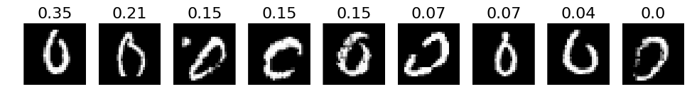
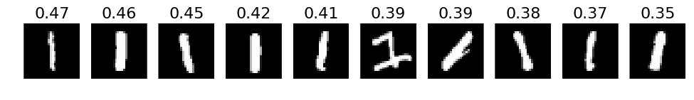
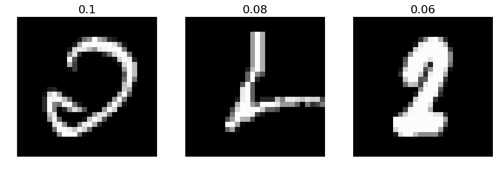
# 4. The most incorrect labels (i.e. those with the highest probabilities that are incorrect)
def incorrect_labels(target_label, nr_sample):
    incorrect = np.where(labels_pred != labels)
    X_incorrect = X_val[incorrect]
    y_incorrect = y_test[incorrect]
    pred_incorrect = predictions[incorrect]

    with_label = np.where(y_incorrect == target_label)
    X_incorrect_with_label = X_incorrect[with_label]
    y_incorrect_with_label = y_incorrect[with_label]
    pred_incorrect_with_label = pred_incorrect[with_label]

    selected = np.argsort(pred_incorrect_with_label[:, target_label])[::-1][:nr_sample]
    plots(X_incorrect_with_label[selected][:nr_sample], titles=np.round(pred_incorrect_with_label[selected][:, target_label][:nr_sample], decimals=2))


# Print for all lables
for i in xrange(10):
    incorrect_labels(i, 10)

Comments