RetinaFace
#ml #dl #face #detection #image #processing
20200903232600
As explained in ([[20200815172158]] Detecting faces from images) detecting faces in a still image is an important step that has various applications.
As of now, a top of the SoTA on face detection can be found on the PapersWithCode website and the best approach seems to be the RetinaFace architecture that we discuss in this section.
The source code for the original paper was published at this github repository with a video for a conference presentation.
It is unfortunately written in MXNet ( #amazon’s #deep #learning framework) but other rewrites are also available:
- In PyTorch
- In Keras + Tensorflow
- A newer Tensorflow 2.0 implementation
- this one, I was actually able to make it work!
The authors of #retinaface originally worked on the more broader problem of #face #recognition so this step is just a precursor to their other model #arcface ([[20200903233242]] ArcFace).
It uses the idea of image #pyramids (convolutions at multiple levels)
There is also a startup around this paper named insightface.ai.
Architecture and paper analysis
The contributions of this paper are:
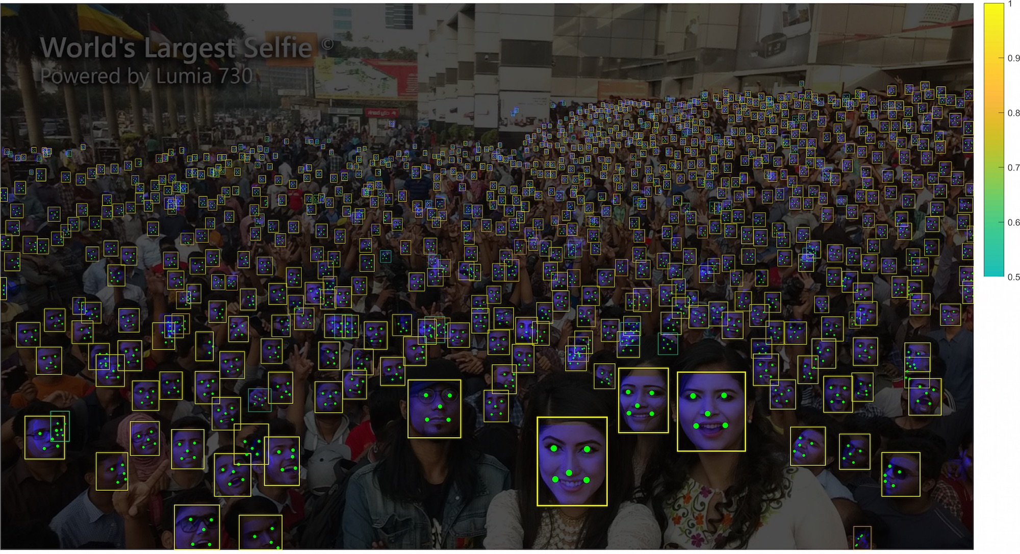
- Creates a a dataset where more features are annotated in multiple faces:
- 5 landmark points: 2 centre of eyes, 2 edges of lips, centre of nose
- a 3D pose matrix specifying how each face is positioned in space
The model is trained to predict simultaneously:
- Whether the current detection is a face or not (binary classification trained using softmax)
- 5 Landmark points
- 3D pose of the face
Loss function
The loss function is a composition of the losses for all 3 detection objectives above:
\[\begin{aligned} Loss = & \> \> \> \> \> \> \> \> \> \> \> \> \> \> {\color{red}Loss_{Classification}}(p_i, p_i^*) + \\ &\lambda_1(=0.25){\color{red}p_i^*}*{\color{blue}Loss_{RegressionBox}}(t_i, t_i^*) + \\ &\lambda_2(=0.1){\color{red}p_i^*}*{\color{green}Loss_{LandmarkPoints}}(l_i, l_i^*) + \\ &\lambda_3(=0.01){\color{red}p_i^*}*{\color{gray}Loss_{3DPixelPose}} \end{aligned}\]\({\color{red}Loss_{Classification}}(p_i, p_i^*)\) is the classification loss where \(p_i\) is the predicted probability of anchor i to being a face and \(p_i^*\) is 1 for the positive anchor (an anchor that is indeed a face) and 0 for the negative anchor (an anchor that is not a face). The classification is a binary crossentropy (they say it’s the softmax loss for binary classes).
\({\color{blue}Loss_{RegressionBox}}(t_i, t_i^*)\) where \(t_i=\{t_x, t_y, t_{height}, t_{width}\}_i\) is the predicted box and \(t_i^*=\{t_x^*, t_y^*, t_{height}^*, t_{width}^*\}_i\) is the ground truth box associated with the positive anchor. The function \({\color{blue}Loss_{RegressionBox}}(t_i, t_i^*)=RobustLoss(t_i, t_i^*)\) where \(R\) is the robust loss function (first defined in Fast R-CNN). The #robust loss function is defined as:
- \[RobustLoss(t_i, t_i^*) = \sum_{j \in \{x, y, w, h\}}smooth_{L1}(t_{ij} - t_{ij}^*)\]
- and \(smooth_{L1}\) is
-
\(smooth_{L1}(x)=0.5x^2\) if $$ x < 1$$ - \(smooth_{L1}(x) = |x| - 0.5\) otherwise. Since all the values of \(t_i\) and \(t_i^*\) are continuous, each one is normalised using a standard scaler (mean=0, std=1) - at train time, as a preprocessing step.
-
\({\color{green}Loss_{LandmarkPoints}}(l_i, l_i^*)\) where \(l_i = \{l_{x1}, l_{y1}, …, l_{x5}, l_{y5}\}_i\) is the predicted 5 facial landmarks, and \(l_i^* = \{l_{x1}^*, l_{y1}^*, …, l_{x5}^*, l_{y5}^*\}_i\) represent the ground-truth associated with the positive anchor. Again, since all the values of \(l_i\) and \(l_i^*\) are continuous, each one is normalised using a standard scaler (mean=0, std=1).
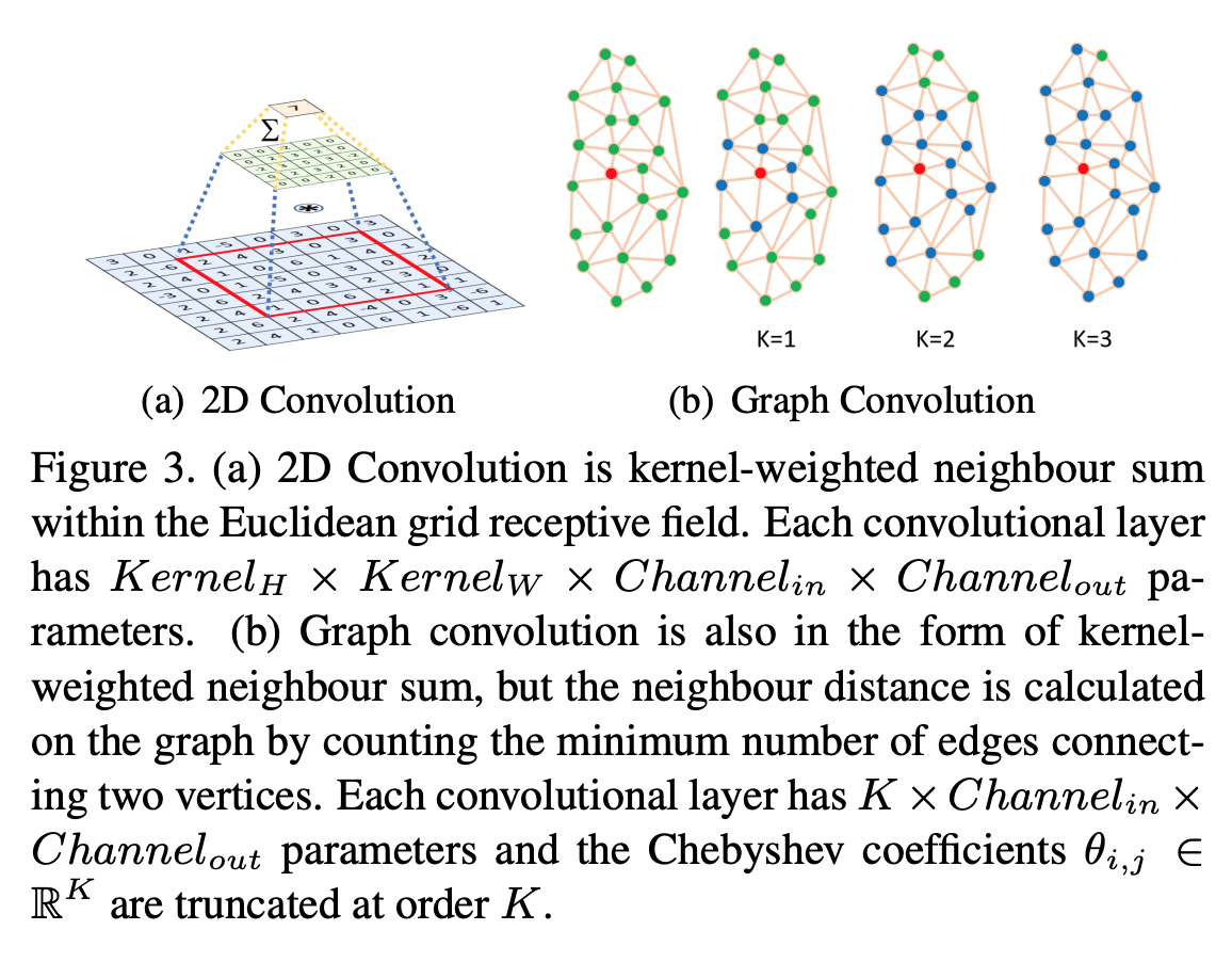
\({\color{gray}Loss_{3DPixelPose}}\) is a loss based on the #graph-convolutional-networks of the ideal face mesh and the current prediction ( [[20200820200300]] Graph Convolutional Networks ) over a 3DMM ( discussed in [[20200825140617]] 3D Morphable Models ), where you have a mesh of a generic person and try to morph that face template so as the projected 2D image matches your target image.
 After estimating the face \((S, T)\) (shape and texture parameters), \(P\) (the projection, or \((camera\_location, camera\_pose, camera\_focal\_length)\) triple ) of the faces, and \(I\) (the illumination properties, i.e. location of point light source, colour values and colour of ambient lighting), they use a fast differentiable 3D mesh renderer for converting the expressed 3D face (given by \((S,T, P, I)\)) onto a 2D projection (I don’t fully understand why they need a differentiable rendered or what does that imply).
The 3D mesh renderer used was published in the 2018 paper titled “Unsupervised Training for 3D Morphable Model Regression” by Google, where they present an end-to-end network that can learn unsupervised 3D faces from images. This paper presents an auto-encoder architecture, which takes and image, converts it to an embedding (via FaceNet or #vgg-face), then pass that embedding to a 3DMM decoder that outputs a 3D image, feed that 3D image in the differentible renderer to get a 2D image (projection) which is compared (via a loss function - this bit simplifying things) to the initial image, and the errors are backpropagated on the full architecture. So we have:
- FaceNet(Target 2D Image) => #face-embedding
- 3DMM(Face-Embedding) => 3D object
- Renderer(3D object) => Predicted 2D Image
- Loss(Target 2D Image, Predicted 2D Image)
The Renderer needs to be differentiable in order to for this system to be an end-to-end trainable one (all the pieces need to be differentiable).
The authors of RetinaNet reused only the Renderer to incorporate it into their network, because they replace Google’s 3DMM step, with one based on the mesh convolutions (via graph convolutions). The basic idea though is that this step takes an input image and outputs a tuple \((S, T, P, I)\) for shape, texture, pose, illumination which is then decoded into a 2D image via Google’s renderer.
Google’s 3DMM decoder uses a 2-layer NN to transform the embeddings into s and t parameters that can be fed into the Basel Face Model 2017 3DMM. This makes Google’s approach really specific to faces, while (I believe) that the mesh convolutions approach can be applied to any known regular object (like #books) as long as you can map them to a class of 3D morphable objects.
From the 2D image obtained in this way, and the target image a MSE (or something similar) is computed for the \({\color{gray}Loss_{3DPixelPose}}\) value.
A Dockerized container
This repository contains a #docker-ized container. Based on their experiments, processing a 3 minutes video on a nVidia 1080Ti GPU enabled computer takes around 15 minutes.
After spending multiple days trying to make it work, I gave up. This was mostly due to the following reasons:
- all the official MxNet CUDA 10.0.x compatible base docker images (other than the nightly build) found on Docker Hub issued
Illegal instruction (core dumped)error when importing the mxnet library - A single official base docker image worked (the nightly build) on loading the mxnet library, but:
- it had python3 installed so:
- I had to update the
Dockerfile(use cython3, and all python3 dependencies) - I had to change the
Makefileto use cython3 to make this build
- I had to update the
- it had mxnet 2.0 (which is only on master and not stable)
- which doesn’t have (yet)
mxnet.mod.Moduleclass which is needed to load the saved model. This class should (supposedly) be implemented in themxnet.modulepackage but this isn’t available yet - there were some discussions on the official GitHub repo that it might be possible to update the load script by using something called
TensorRTby going from:
- which doesn’t have (yet)
- it had python3 installed so:
self.model = mx.mod.Module(symbol=sym, context=self.ctx, label_names = None)
to
os.environ['MXNET_USE_TENSORRT'] = '1'
trt_sym = sym.get_backend_symbol('TensorRT')
mx.contrib.tensorrt.init_tensorrt_params(trt_sym, arg_params, aux_params)
mx.contrib.tensorrt.set_use_fp16(False)
self.model = trt_sym.simple_bind(ctx=self.ctx, data = (1,3,image_size[0], image_size[1]), grad_req='null', force_rebind=True)
    * But:
        * this isn't enabled by default and need a source recompilation of mxnet with some flag enabled (`USE_TENSORRT=1`) which defeats the whole purpose of using a prebuild official docker container for mxnet in the first place..
Another Dockerized container
Docker comtainer can be found here( mlouieunm/insightface-vj ), with a brief video explanation of how it works here (https://www.youtube.com/watch?v=aP8WCgKbIXc). From what I see it requires CUDA 10.1 which isn’t installed on the machine that I have..

Comments