Cluj ml enthusiasts

My last post received quite some responses, but before actually settling on the curricula of the upcoming ML course, I’ve decided to “eat my own lunch” and use ML to analyze what the data is telling me.

More specifically I’m interested in the classes of ML enthusiasts that exist in Cluj-Napoca, and try to identify what those classes represent. I’d like to understand who my audience is, what they know, and what they’d like to learn next.

I’d also like to get an insight into why are they interested in joining this course.

The basic strategy that I’m going to use, is:

• data cleaning
• feature engineering
• feature analysis
• clustering
• cluster analysis

In the end I’ll end up with the insight I’m seeking, so let’s proceed!

Load the data

Code

%matplotlib inline
import sklearn 
import pandas as pd
import numpy as np
from matplotlib import pyplot as plt

I have a WorkAt field that I’m going to drop it as it contains sensitive information.

Code

df = pd.read_csv("Cluj_ML_Enthusiasts.csv", sep='\t', na_values=['-']).drop(columns=['Email address', 'Name'])
df.drop(columns=['WorkAt']).head()

	Timestamp	Knowledge	Effort	Degree	IsResearcher	IsML	IsDeveloper	IsTeaching	IsStudent
0	29/10/2018 16:05:09	15	16	4	True	True	True	False	False
1	29/10/2018 16:11:16	7	32	3	False	False	True	False	False
2	29/10/2018 17:18:45	6	16	3	False	False	True	False	False
3	29/10/2018 17:21:18	6	4	3	False	False	True	False	False
4	29/10/2018 17:25:51	10	4	3	False	True	True	False	False

The Knowledge field contains values that represent, in ascending order, the self-assessment of ML knowledge. The actual number-to-question relation is found bellow:

1 - I heard about ML
2 - I understand what ML is and should be doing
3 - I've used some packaged libraries / API's that used ML in the background 
4 - I regularly read news articles or blogs about ML and wish to transition into ML
5 - I've started online ML courses but gave up before finishing
6 - I've finished 1-2 courses about ML (at university or online)
7 - I've followed a few tutorials and executed their code ony my machine / forked the GitHub project
8 - I've registered on Kaggle and ran some kernels other people wrote
9 - I've wrote some ML hobby projects / played with some Kaggle datasets myself
10- I've been recently employed on an ML position
11- I've finished a PoC ML code for my employer but the project is young
12- I know how to debug my ML model, I understand what it does and what are it's shortcomings
13- I know the academic name, SoTA, previous work for the class of problems that I work on.
14- I've competed and finished in top 10% in at least one Kaggle competition / I have active ML code in production
15- I read ML academic papers and am trying to reproduce their results / Pursuing or have a PhD in AI
16- I'm able to reproduce ML academic papers and can evaluate the correctness of their claims
17- When I read a paper I can easily see where this fits in the current SoTA, and can anticipate some future directions of research
18- I write ML papers with code released online that gets published in recognized venues / I work at DeepMind, FAIR or Microsoft Research

The Degree field is a 4 value list for the following enumeration:

1 - Student
2 - BsC
3 - MsC
4 - PhD

The other Is.. fields are just expansions of the information contained in Knowledge, Degree and WorkAt columns taken as a whole which I’ve filled them myself.

Clean the data

Making the WorkAt column a categorical column. This both hides the sensitive information while at the same time, converts everything into numbers. ML models love numbers!

Code

df.WorkAt = df.WorkAt.astype('category').cat.as_ordered().cat.codes + 1

Making a numerical copy of the dataframe and anonymising the data

Code

df_num = df.copy()
df_num.WorkAt = df.WorkAt.astype('category').cat.as_ordered().cat.codes + 1
df_num.tail()

	Timestamp	Knowledge	Effort	Degree	IsResearcher	IsML	IsDeveloper	IsTeaching	IsStudent	WorkAt
67	01/11/2018 16:26:09	12	4	3	True	True	False	True	False	21
68	02/11/2018 09:20:57	1	16	2	False	False	True	False	False	22
69	02/11/2018 22:25:43	2	16	1	True	False	False	True	False	20
70	02/11/2018 22:29:13	2	16	3	False	False	True	False	False	13
71	06/11/2018 22:14:40	5	16	1	False	False	False	False	True	21

Converting the Timestamp column to datatime. This needs some attention and this case a specific format parameter was required for pandas. It usually infers the date format correctly but in this instance some of the November entries were detected as being from February.

Code

df_num.Timestamp = pd.to_datetime(df_num.Timestamp, dayfirst=True, format="%d/%m/%Y %H:%M:%S")

Some feature engineering

Adding an HoursElapsed column, infered from the Timestamp column. The HoursElapsed represent a synthetic feature that counts the number of hours passed between me publishing the news and the actual registration. It’s usefull to know how fast a certain user reacted when seeing the event.

Code

import numpy as np
hours_elapsed = df_num.Timestamp.astype(np.int64) // ((10 ** 9) * 3600) # hours
hours_elapsed -= min(hours_elapsed)
df_num['HoursElapsed'] = hours_elapsed
df_num.head()

	Timestamp	Knowledge	Effort	Degree	IsResearcher	IsML	IsDeveloper	IsTeaching	IsStudent	WorkAt	HoursElapsed
0	2018-10-29 16:05:09	15	16	4	True	True	True	False	False	6	0
1	2018-10-29 16:11:16	7	32	3	False	False	True	False	False	6	0
2	2018-10-29 17:18:45	6	16	3	False	False	True	False	False	10	1
3	2018-10-29 17:21:18	6	4	3	False	False	True	False	False	17	1
4	2018-10-29 17:25:51	10	4	3	False	True	True	False	False	18	1

The HoursElapsed per se, are just a quick proxy for measuring how enthusiastic is a certain user about the idea of an ML course. Arguably, it’s also a proxy of how much time he/she spends on Facebook or Twitter, but I’ll assume the former.

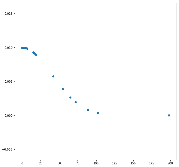
I’ll do a simple transformation on the HourElapsed by which most recent ones will have a high number and the more distant ones will fade to 0 enthusiasm.

Modeling the enthusiasm of people by assuming that the velocity of their response is relative to a positive Gaussian kernel, that defines the Enthusiasm

Code

from math import pi
plt.rcParams['figure.figsize'] = [10, 10]

def gaussian(x, std): 
    return np.exp(-0.5*((x/std)**2)) / (std * np.sqrt(2*pi))


from matplotlib import pyplot as plt
plt.scatter(df_num.HoursElapsed, gaussian(df_num.HoursElapsed, 40))

We are going to add the Enthusiasm values to our data, bellow.

Code

kernel = gaussian(df_num.HoursElapsed, 40)
kernel = (kernel - kernel.mean()) / kernel.std()
kernel

df_num['Enthusiasm'] = kernel
df_num.tail()

	Timestamp	Knowledge	Effort	Degree	IsResearcher	IsML	IsDeveloper	IsTeaching	IsStudent	WorkAt	HoursElapsed	Enthusiasm
67	2018-11-01 16:26:09	12	4	3	True	True	False	True	False	21	72	-1.789470
68	2018-11-02 09:20:57	1	16	2	False	False	True	False	False	22	89	-2.122546
69	2018-11-02 22:25:43	2	16	1	True	False	False	True	False	20	102	-2.255501
70	2018-11-02 22:29:13	2	16	3	False	False	True	False	False	13	102	-2.255501
71	2018-11-06 22:14:40	5	16	1	False	False	False	False	True	21	198	-2.368870

Now that we’ve added the Enthusiasm column, we can remove the HoursElapsed and Timestamp columns since they are correlated with the Enthusiasm

Code

df_num = df_num.drop(columns=['Timestamp', 'HoursElapsed'])

Feature analisys

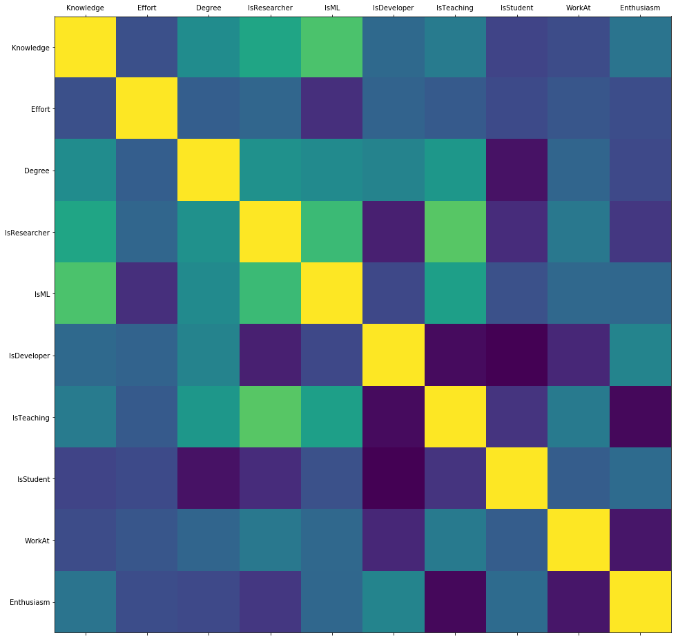
Do a feature analysis and remove highly correlated features

Code

def plot_correlation(df_num):
    plt.rcParams['figure.figsize'] = [140, 105]
    corr = df_num.corr().abs()
    plt.matshow(df_num.corr())
    plt.xticks(ticks=np.arange(len(df_num.columns.values)), labels=df_num.columns)
    plt.yticks(ticks=np.arange(len(df_num.columns.values)), labels=df_num.columns)
    plt.show()
    return corr

corr = plot_correlation(df_num)

Code

# https://stackoverflow.com/questions/17778394/list-highest-correlation-pairs-from-a-large-correlation-matrix-in-pandas
def get_redundant_pairs(df):
    '''Get diagonal and lower triangular pairs of correlation matrix'''
    pairs_to_drop = set()
    cols = df.columns
    for i in range(0, df.shape[1]):
        for j in range(0, i+1):
            pairs_to_drop.add((cols[i], cols[j]))
    return pairs_to_drop

def get_top_abs_correlations(df, n=5):
    au_corr = df.corr().abs().unstack()
    labels_to_drop = get_redundant_pairs(df)
    au_corr = au_corr.drop(labels=labels_to_drop).sort_values(ascending=False)
    return au_corr[0:n]

get_top_abs_correlations(df_num, n=20)

IsResearcher  IsTeaching      0.624758
Knowledge     IsML            0.585793
IsResearcher  IsML            0.535484
IsDeveloper   IsStudent       0.452602
IsTeaching    Enthusiasm      0.422794
IsDeveloper   IsTeaching      0.408248
Knowledge     IsResearcher    0.402911
Degree        IsStudent       0.384491
IsML          IsTeaching      0.369175
WorkAt        Enthusiasm      0.363629
IsResearcher  IsDeveloper     0.324617
Degree        IsTeaching      0.315283
IsDeveloper   WorkAt          0.293584
Degree        IsResearcher    0.282929
IsResearcher  IsStudent       0.266398
Effort        IsML            0.254194
Knowledge     Degree          0.253271
Degree        IsML            0.239952
IsTeaching    IsStudent       0.234521
IsResearcher  Enthusiasm      0.219462
dtype: float64

We can see that some of the pairs are highly correlated with the other. From the mostly correlated pairs we’re going to drop one of them, as it contains redundant information.

Decided on dropping the following columns:

IsML, Degree, IsResearcher

In addition, WorkAt brings no evident value, drop it.

Code

df_num = df_num.drop(columns=['IsML', 'Degree', 'IsResearcher', 'WorkAt'])
df_num.head()

	Knowledge	Effort	IsDeveloper	IsTeaching	IsStudent	Enthusiasm
0	15	16	True	False	False	0.558944
1	7	32	True	False	False	0.558944
2	6	16	True	False	False	0.558029
3	6	4	True	False	False	0.558029
4	10	4	True	False	False	0.558029

Data plotting

We will attempt to plot the data that we have on a 2D plot. In order to do this, we will reduce the dimensionality of it using PCA. This is useful because we want to get a rough idea of how many clusters do we have.

Code

from sklearn.pipeline import Pipeline
from sklearn.preprocessing import StandardScaler
from sklearn.cluster import AffinityPropagation, AgglomerativeClustering, KMeans

from sklearn.decomposition import PCA


pipe = Pipeline([
    ('scaler', StandardScaler()),
    ('dim_reducer', PCA(n_components=2))
])


reduced = pipe.fit_transform(df_num.values.astype(np.float32))

plt.rcParams['figure.figsize'] = [10, 10]
plt.scatter(reduced[:, 0], reduced[:, 1])

for i, (x, y) in enumerate(reduced[:, [0, 1]]):
    plt.text(x, y, "Name " + str(df.index[i]))

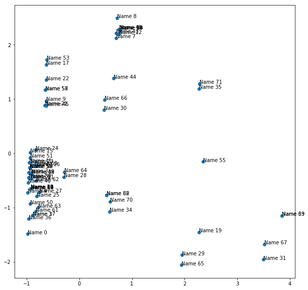
If you squint, it seems we have roughly 4 generic clusters (with a couple of outliers). We will use KMeans clustering with this value, but only after we normalize all the features. Let’s see what we get!

Code

df_ = df_num.copy()
pipe = Pipeline([
    ('scaler', StandardScaler()),
    ('cluster', KMeans(n_clusters=4))
])

df_['Cluster'] = pipe.fit_predict(df_num)
df_.sort_values('Cluster')

	Knowledge	Effort	IsDeveloper	IsTeaching	IsStudent	Enthusiasm	Cluster
0	15	16	True	False	False	0.558944	0
36	12	16	True	False	False	0.558944	0
32	1	16	True	False	False	-2.122546	0
37	7	32	True	False	False	0.558944	0
38	3	16	True	False	False	0.558029	0
27	6	16	True	False	False	0.246598	0
25	7	16	True	False	False	0.333842	0
42	3	16	True	False	False	0.558029	0
63	9	16	True	False	False	0.246598	0
45	7	16	True	False	True	0.555286	0
46	6	16	True	False	False	0.555286	0
47	6	16	True	False	False	0.555286	0
34	4	16	True	False	False	-2.255501	0
50	9	16	True	False	False	0.544341	0
49	3	16	True	False	False	0.550721	0
6	4	16	True	False	False	0.558029	0
1	7	32	True	False	False	0.558944	0
2	6	16	True	False	False	0.558029	0
61	10	16	True	False	False	0.333842	0
14	6	16	True	False	False	0.544341	0
68	1	16	True	False	False	-2.122546	0
70	2	16	True	False	False	-2.255501	0
10	6	16	True	False	False	0.555286	0
11	4	16	True	False	False	0.555286	0
13	6	16	True	False	False	0.550721	0
9	6	16	True	False	True	0.555286	0
64	3	4	True	False	False	-0.681784	1
53	1	4	True	False	True	0.536159	1
41	4	4	True	False	False	0.558029	1
62	7	4	True	False	False	0.277015	1
...	...	...	...	...	...	...	...
24	1	4	True	False	False	0.360152	1
23	4	4	True	False	False	0.514453	1
22	5	4	True	False	True	0.514453	1
21	10	4	True	False	True	0.514453	1
3	6	4	True	False	False	0.558029	1
4	10	4	True	False	False	0.558029	1
17	2	4	True	False	True	0.536159	1
16	5	4	True	False	False	0.536159	1
15	2	4	True	False	False	0.544341	1
5	7	4	True	False	False	0.558029	1
55	1	4	False	True	False	0.526190	2
31	15	4	False	True	False	-1.789470	2
67	12	4	False	True	False	-1.789470	2
33	2	16	False	True	False	-2.255501	2
19	15	4	False	True	False	0.526190	2
65	5	16	True	True	False	-1.231252	2
69	2	16	False	True	False	-2.255501	2
29	3	16	True	True	False	-1.231252	2
35	6	16	False	False	True	-2.368870	3
54	1	16	False	False	True	0.526190	3
48	1	16	False	False	True	0.550721	3
44	14	4	False	False	True	0.558029	3
43	5	4	False	False	True	0.558029	3
20	1	16	False	False	True	0.526190	3
18	1	16	False	False	True	0.526190	3
12	2	16	False	False	True	0.550721	3
8	2	4	False	False	True	0.558029	3
7	6	4	False	False	True	0.558029	3
56	1	16	False	False	True	0.526190	3
71	5	16	False	False	True	-2.368870	3

72 rows × 7 columns

From the initial looks of it, the clusters have the following characteristics:

• 0 - High commitment Developers (36,1%)
• 1 - Quick win Developers (36,1%)
• 2 - Academics / Researchers (11,1%)
• 3 - Unemployed students (16,7%)

AffinityPropagation is a clustering algo that doesn’t require a number of clusters as its inputs. I’m going to use it for estimating the number of clusters, because maybe I’m missing some clusters.

Code

nr_clusters = np.unique(AffinityPropagation().fit_predict(df_num))
nr_clusters

array([0, 1, 2, 3, 4])

It seems that there’s roughly the same amount of clusters that it finds. After some inspection, it seems that the model decided to split the ‘Accademics’ into high and low commitment ones.

• 1 - Quick win Developers ( 36,1% )
  • < 4h work / week
  • employed

• 2 - Unemployed students ( 16,7% )

• 3 - High commitment Developers ( 36,1% )
  • 16+ hours / week
  • employed
• 4 - Academics ( 11,1% )
  • high commitment (> 16h/week) ( 5,6% )
  • low commitment (< 4h/week) ( 5,6% )

So there you go! I won’t draw any conclusions to the above findings, I’ll leave the interpretation of the result up to you, but people seem generally interested in ML ;)